-
Články
- Vzdělávání
- Časopisy
Top články
Nové číslo
- Témata
- Kongresy
- Videa
- Podcasty
Nové podcasty
Reklama- Kariéra
Doporučené pozice
Reklama- Praxe
Estimating Divergence Time and Ancestral Effective Population Size of Bornean and Sumatran Orangutan Subspecies Using a Coalescent Hidden Markov Model
Due to genetic variation in the ancestor of two populations or two species, the divergence time for DNA sequences from two populations is variable along the genome. Within genomic segments all bases will share the same divergence—because they share a most recent common ancestor—when no recombination event has occurred to split them apart. The size of these segments of constant divergence depends on the recombination rate, but also on the speciation time, the effective population size of the ancestral population, as well as demographic effects and selection. Thus, inference of these parameters may be possible if we can decode the divergence times along a genomic alignment. Here, we present a new hidden Markov model that infers the changing divergence (coalescence) times along the genome alignment using a coalescent framework, in order to estimate the speciation time, the recombination rate, and the ancestral effective population size. The model is efficient enough to allow inference on whole-genome data sets. We first investigate the power and consistency of the model with coalescent simulations and then apply it to the whole-genome sequences of the two orangutan sub-species, Bornean (P. p. pygmaeus) and Sumatran (P. p. abelii) orangutans from the Orangutan Genome Project. We estimate the speciation time between the two sub-species to be thousand years ago and the effective population size of the ancestral orangutan species to be , consistent with recent results based on smaller data sets. We also report a negative correlation between chromosome size and ancestral effective population size, which we interpret as a signature of recombination increasing the efficacy of selection.
Published in the journal: . PLoS Genet 7(3): e32767. doi:10.1371/journal.pgen.1001319
Category: Research Article
doi: https://doi.org/10.1371/journal.pgen.1001319Summary
Due to genetic variation in the ancestor of two populations or two species, the divergence time for DNA sequences from two populations is variable along the genome. Within genomic segments all bases will share the same divergence—because they share a most recent common ancestor—when no recombination event has occurred to split them apart. The size of these segments of constant divergence depends on the recombination rate, but also on the speciation time, the effective population size of the ancestral population, as well as demographic effects and selection. Thus, inference of these parameters may be possible if we can decode the divergence times along a genomic alignment. Here, we present a new hidden Markov model that infers the changing divergence (coalescence) times along the genome alignment using a coalescent framework, in order to estimate the speciation time, the recombination rate, and the ancestral effective population size. The model is efficient enough to allow inference on whole-genome data sets. We first investigate the power and consistency of the model with coalescent simulations and then apply it to the whole-genome sequences of the two orangutan sub-species, Bornean (P. p. pygmaeus) and Sumatran (P. p. abelii) orangutans from the Orangutan Genome Project. We estimate the speciation time between the two sub-species to be thousand years ago and the effective population size of the ancestral orangutan species to be , consistent with recent results based on smaller data sets. We also report a negative correlation between chromosome size and ancestral effective population size, which we interpret as a signature of recombination increasing the efficacy of selection.
Introduction
There is a growing awareness that the genomic sequences now available for closely related species or sub-species may provide detailed information on the population genetics process in the ancestors of these species and about the speciation process itself [1]. This is because the divergence patterns of a set of (sub-)species vary along their genomes due to polymorphism in the ancestral species. Different parts of the genome have different histories because recombination has brought together the genome from different ancestors. Viewed back in time, two sequences are therefore, at any given point in the genome, a sample of two individuals in the ancestral species and the identity of these individuals vary along the sequence, as illustrated in Figure 1. The varying sequence-divergence times provide information that allows us to examine the speciation process [2], [3] and enable inference of parameters for the population genetics of the ancestral species, such as the effective population size or speciation-divergence or population-divergence times [4]–[6].
Fig. 1. The ancestry of two genomic sequences. 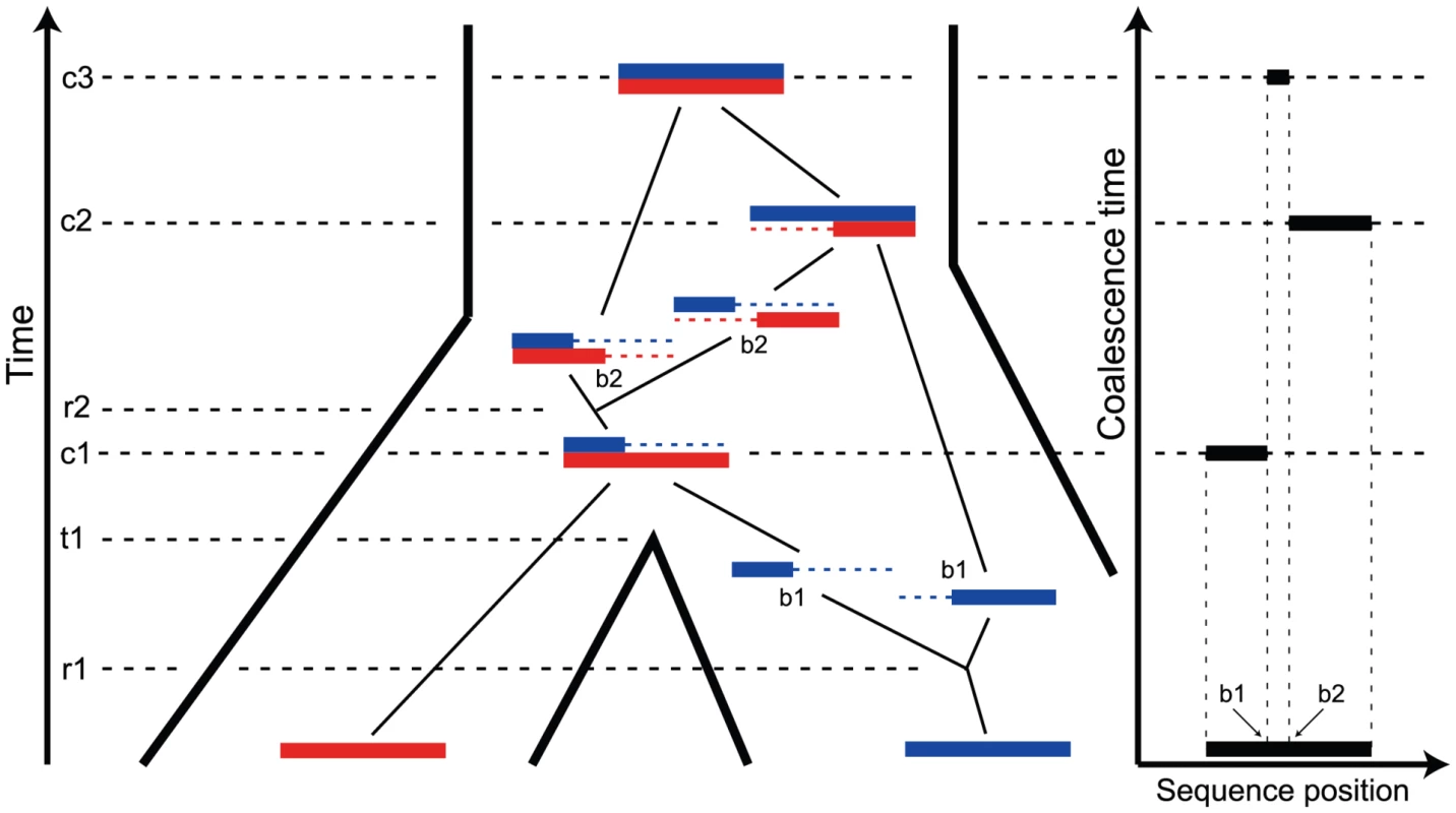
The figure illustrates the ancestry of two genomic sequences (in red and blue) from two different populations. Tracing their ancestry back in time, the first event we see is a recombination (at time and sequence position ) within the “blue population”. This is followed by the population split (at time ), and thus the “red genome” enters the ancestral population as a contiguous segment, while the “blue genome” enters the ancestral population in two fragments. The process in the ancestral population now under goes coalescence events (at times , , and ) and a recombination event (at time and sequence position ). A consequence of the coalescence process with recombination is that the coalescence times, and thus the sequence divergence, changes along the genomic alignment at the recombination break points (illustrated on the right). Coalescent theory [7] tells us that the variation in coalescence time in an ancestral population is directly proportional to the effective population size of the ancestral population. This was exploited by Takahata [8] in order to derive a simple estimator of the ancestral effective population size, but when applied to human and chimpanzee the estimate was associated with a large variance, because of the limited divergence of these species. Takahata [9] showed that including an outgroup improved the results, and Yang [10] showed that mutation rate heterogeneity is confounded with the estimate. These early approaches estimated a fixed phylogeny for different sequence fragments. Later approaches have exploited the fact that if speciation times are sufficiently close together, incomplete lineage sorting (cases where the gene tree is different from the species tree) may occur. Wall [11] allowed for recombination and several species in the likelihood estimation of population parameters and Patterson et al. [2], Hobolth et al. [5], and Dutheil et al. [12] made simple models of changes in genealogy along a multi-species alignment with incomplete lineage sorting.
Detailed modeling using MCMC of the genealogies supporting a data set [13], or the ancestral recombination graph [3] in a model that includes recombination, has the advantage of allowing modeling more complex aspects of the data such as gene flow through migration, but scaling these to whole genome data is challenging. In contrast, approaches based on hidden Markov models (HMMs), such as Hobolth et al. [5], and Dutheil et al. [12], provide computationally fast inference algorithms, which are scalable to whole-genome data sets. Nevertheless, modeling complex demographic models in terms of transition matrices and emission probabilities is mathematically challenging.
Here we present a new approach for constructing transition matrices for HMM approaches and use it to capture the variation in coalescence time between the genomes of two individuals from two divergent populations or two closely related species. The model traces the ancestry of the two sequences using the coalescence process with recombination [14]–[16], and this process determines the switching probabilities from one coalescent time to another along the pair of sequences. Considering a junction between two nucleotides, and going back in time, two types of events may occur: a sequence can split up in two fragments (a recombination event) and two fragments can merge again to become one (a coalescence event). We model the two species using an isolation model (recall Figure 1). Initially, the sequences from the two populations evolve independently, meaning that coalescence events always involves sequences from within the same population. After the population split event, the two populations become one, and the two (fragmented) sequences can now start finding most recent common ancestors. As a result of these events, the sequence divergence varies as we scan along the genomic sequences. The patterns of sequence divergence, and the distribution of recombination events separating segments with constant divergence, are informative of the coalescent processes in the separate populations and that of the ancestor.
The model is parameterized with the split time between the two populations, the effective population size of the ancestral population, and the recombination rate, which is assumed to be constant along the segment of the genome analysed. The model assumes that no migration occurs after the population split. We validate the model by simulations and then apply it to the recently sequenced genomes of the two orangutan subspecies Bornean (P. p. pygmaeus) and Sumatran (P. p. abelii) [17]. We estimate the sub-species divergence time to be thousand years ago (kya), and the effective population size of the ancestral orangutan to be estimated from the autosomal chromosomes, and about of that for the X chromosome: .
Results
A coalescent time hidden Markov model
We have developed a new coalescent hidden Markov model (CoalHMM). The properties characterizing CoalHMMs [5], [12] are that they model the coalescent process as a Markov process along an alignment, and conditional on the alignment can infer the unobserved genealogies that lead to the alignment, or integrate over the distribution of genealogies. While the coalescent process is only Markovian in time but not in space [16], [18], we have previously shown that we can reasonably approximate it as a Markov process along the sequence [12], [19], [20] and doing this enables us to develop very efficient inference algorithms compared to the sampling based approaches usually needed to capture the true coalescent process.
The crux of developing a CoalHMM is specifying the transition probabilities of the hidden Markov model in terms of the coalescent process parameters, e.g. recombination rates and effective population sizes. In Hobolth et al. [5], this issue was largely ignored and coalescent parameters were obtained from post-processing of inferred hidden Markov model parameters. In Dutheil et al. [12] the transition probabilities were derived from the coalescent process through a set of rather complicated equations and simplifying assumptions. The approach we describe in this paper greatly simplifies the computation of transition probabilities and does so without simplifying assumptions beyond assuming that the process is Markovian along the alignment.
The key insight behind our new approach, also observed in Dutheil et al. [12], is that since we assume that the process is Markovian along the alignment we need only consider the genealogies of pairs of adjacent nucleotides. The new approach differs from Dutheil et al. in the way we exploit this insight. Here, we explicitly consider the coalescent with recombination process for pairs of nucleotides and derive the exact transition probabilities from this model.
The new approach that allows us to calculate the exact transition probabilities from the coalescence process with recombination differs from the previous CoalHMMs we have developed, where this process has been approximated.
Modeling genealogies as a two-nucleotide coalescent process
In our new CoalHMM approach, we use two different Markov models: one that models the coalescence times along the sequences as a discrete space Markov model, and one that models the ancestry of two neighboring nucleotides back in time as a continuous time, finite state Markov model. The first model is used as the hidden Markov model when estimating parameters, while the second is used to compute the transition probabilities of the first.
The coalescent process, when viewed as a process in time rather than along the alignment, is a continuous time Markov chain (CTMC) on a finite state space. For a single sequence, the two nucleotide CTMC has just two states: the two adjacent nucleotides can be linked, i.e. sitting on the same haploid chromosome, or unlinked, i.e. sitting in two different chromosomes (see Figure 2). A recombination event changes the CTMC from the first state to the second and a coalescent event changes the CTMC from the second state back to the first. The rate of change from the first state to the second is the rate of coalescence events (one coalescent event per generations, where is the effective population size), and the rate of change from the second state to the first is the rate of recombination events.
Fig. 2. States for the single species system. 
For a single species we have two nucleotides, one left and one right, and these can either be linked or unlinked. Assuming that the two nucleotides are initially linked, i.e. that the CTMC is initially in state 1, we can calculate the probability that it is in state 1 or state 2 for any point in time (see Figure 3). This probability distribution will tend toward an equilibrium defined by the ratio between the coalescent rate and the recombination rate. As the coalescence rate is inversely proportional to the effective population size, the larger the effective population size the less likely that the nucleotides are linked at the equilibrium, although in general the CTMC is much more likely to be in the linked state than the unlinked as in general the recombination rate for two neighboring nucleotide is orders of magnitude smaller than the coalescence rate.
Fig. 3. State probabilities for the single sequence two-nucleotide coalescent process as a function of time. 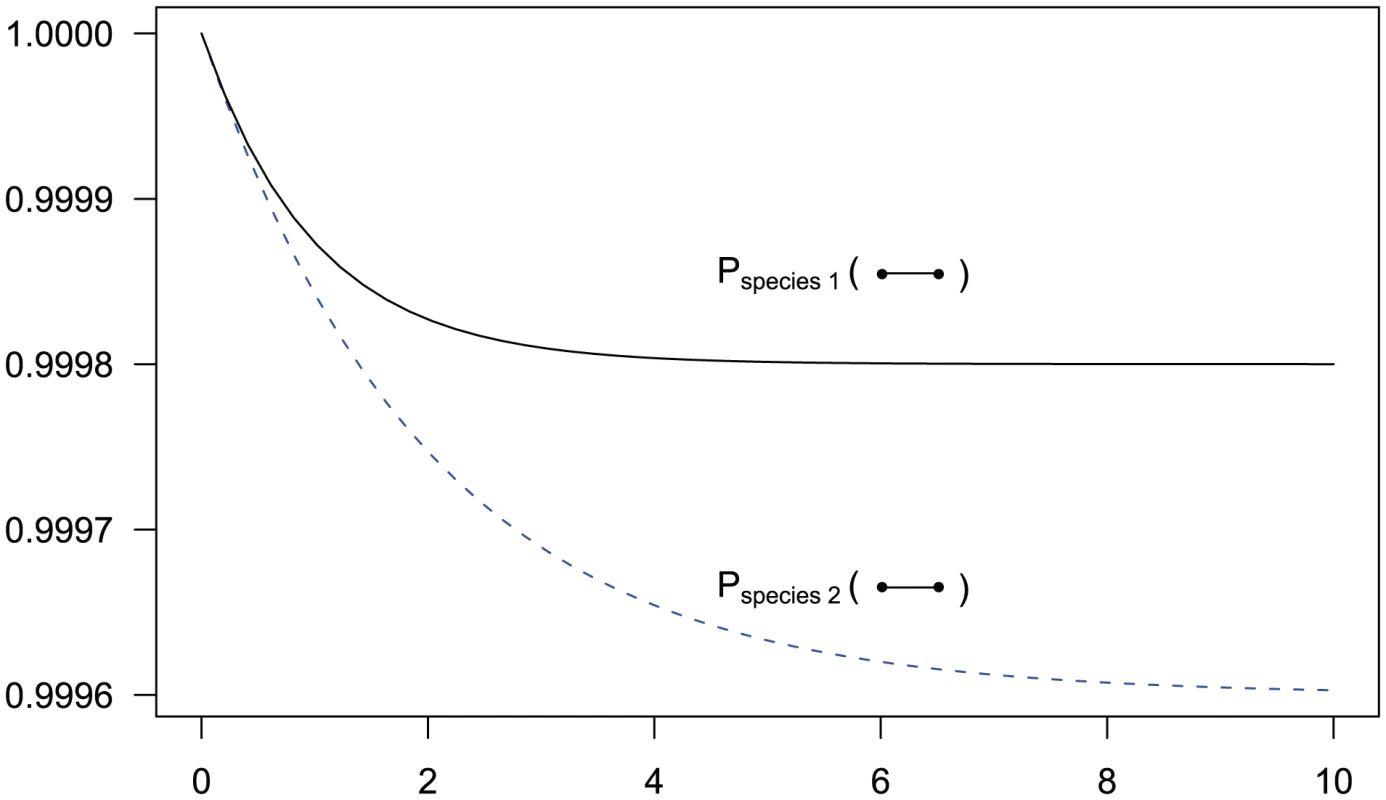
The figure shows the probability of the two neighboring nucleotides being linked in the single-sequence CTMC and how this probability evolves over time. The probability for being unlinked is, of course, one minus the probability of being linked, since the CTMC has only two states. The two different lines correspond to two different coalescence rates. For population 1, the coalescence rate is set to 1 (so the x-axis is in units of generations for this species), while for population 2 the coalescence rate is half that, corresponding to population 2 having twice the effective population size of population 1. The recombination rate is set to . Assuming of 20,000 for population 1 and 40,000 for population 2, and a generation time of 20 years, this corresponds to 1 cM/Mbp and 1 unit on the x-axis corresponds to 400,000 years. The separation time we infer for the orangutan sub-species is around on the x-axis, where the system is still far from equilibrium. For two sequences, the coalescence process we consider contains two adjacent nucleotides from each sequence, and the state space consists of all possible ways that these four nucleotides can be combined: linked or unlinked between left and right nucleotides and having coalesced into their most recent common ancestor or not for nucleotides at the same position. In Figure 4 we have summarized the state space of the system. The 15 states correspond to the various ways the two genomes (the top and the bottom row) can link the left and right nucleotides or be merged in common ancestors (white dots).
Fig. 4. States for the two species system. 
For the two species system, we have one or two left and one or two right nucleotides. One when the left or right nucleotides have found their MRCA (open circles) and two otherwise (filled circles). Left nucleotides can be linked with right nucleotides or not. When modeling the ancestry of one sequence for each of two populations, the system will first evolve independently as two single-sequence CTMCs back in time and then merge into a single two-sequence CTMC with initial probability distribution given by the end-states of the single sequence CTMCs. The two sequences from the single-sequence CTMCs can, after entering the two-sequence CTMC, recombine and coalesce as in the single-sequence CTMC, but now with the possibility of linking the left-nucleotide from one population to the right-nucleotide of the other population. Figure 5 shows the probability distribution of the two-sequence CTMC states for states 1 to 7 (see Figure 4) that corresponds to the states where left and right nucleotides are recombining and coalescing.
Fig. 5. Evolution of states in the two-sequence CTMC. 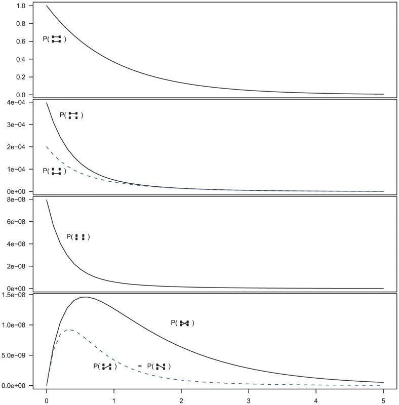
The figure shows the beginning states in the two-sequence CTMC and how their probabilities evolve over time. The asymmetry between which original sequence is linked versus unlinked, when only one sequence is linked (the second plot from the top) is caused by the differences in effective population size within the single-sequence CTMC system used for determining the initial distribution of the two-sequence distribution. The initial probability is taken from the two populations in Figure 3 at time 10 (the right edge of that figure) and the rates in the two-sequence system correspond to those for population 1 in Figure 3, i.e. a coalescence rate of 1 and a recombination rate of . In addition to these events, it is possible for the two left-nucleotides or the two right-nucleotides to coalesce into the most recent common ancestor of the two original sequences. These events are irreversible in the CTMC and eventually both left and right nucleotides have found a most recent common ancestor and the two-sequence CTMC essentially reduces to the single-sequence CTMC.
Calculating transition probabilities from the two-nucleotide coalescent process
From the two CTMC systems we can compute the probability distribution of genealogies of adjacent nucleotides back in time. We use this to construct the second Markov model, a Markov process along the alignment, in the following way: 1) we split the coalescence times back in time into a finite set of time intervals that will be the states of the hidden Markov model along the alignment, 2) for time intervals and we use the CTMC system to compute the probability that the left nucleotides find their most recent common ancestor in interval while the right nucleotides find their most recent common ancestor in interval , and 3). We calculate the transition probability of moving from interval/state to interval/state as .
Of these steps, 1) and 3) are trivial to achieve. Step 2) is achieved by considering four different sub-sets of the two-sequence CTMC: , , and . The first set consists of the states where neither left nor right nucleotide have reached their most recent common ancestor, the next two consist of the states where only the left or only the right, respectively, have reached their most recent common ancestor, and finally the last set consists of the states where both left and right nucleotides have reached their most recent common ancestor. Tracing the history of the nucleotides back in time, all histories begin in a state in and end in . Most histories go directly from to (where both left and right nucleotides coalesce at the same time by being linked at the time they reach their most recent common ancestor) but some find a most recent common ancestor first at the left nucleotide, a state in , or first at the right nucleotide, a state in , before reaching . The probability of being in the four classes of states as a function of time is shown in Figure 6.
Fig. 6. Evolution of the two-sequence CTMC. 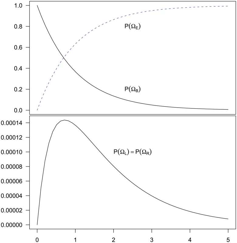
The figure shows how the probability of being in one of the four classes of states evolve over time. Initially, the system is in with probability 1, but this probability drops exponentially. With a relatively small probability the system will go through a state in or before ending up in but mainly states move directly to states. The rate parameters used are the same as those in Figure 5. From the probability distribution of the four state classes back in time, we can construct the joint probability of having the left nucleotide finding its most recent common ancestor in interval and the right nucleotide finding its most recent common ancestor in interval in a straightforward manner (see Methods for details). To get the probability e.g. for we calculate the probability that the system is in until it reaches interval and then is in when it leaves interval (see Figure 7, left). For (and symmetrically for ) we calculate the probability that the system is in until it reaches interval , leaves interval in and stays in until it reaches interval which it leaves in (see Figure 7, right).
Fig. 7. Transition probabilities calculated from the CTMC system. 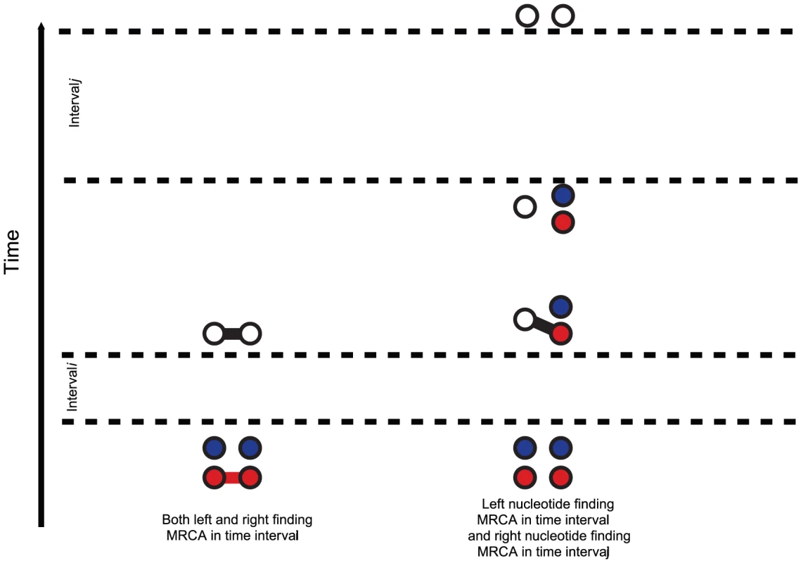
The hidden Markov model transition probabilities are calculated by considering the probabilities, in the two nucleotide CTMC system, that either both left and right nucleotide finds a most recent common ancestor in the same time interval (left) or that the left nucleotide finds a most recent common ancestor in one given interval, , and the right in another, (right). Model validation: simulation study
The power and consistency of the model can be evaluated through simulations. The HMM is designed to approximate the coalescent with recombination process. Thus, we simulate data using a coalescent with recombination and then compare inferred parameters from the HMM model with the values used in the simulations.
We first examined the fit between the coalescent process with recombination and the Markov approximation by examining the empirical distribution of time spent in each time interval with the Markov calculations (see Supplemental Section 1.1 of Protocol S1). Hereafter we estimated the probability of moving from one time interval to another based on simulations and compared that to the transition probabilities in the HMM (see Supplemental Section 1.2 of Protocol S1), and generally a good match between the two was found. Next we computed the likelihood surface for our three main parameters and inspected these manually. Generally we found the maximum likelihood near the true value for all three parameters, but with a rather flat likelihood for the recombination rate parameter (see Supplemental Section 1.3 of Protocol S1).
Most important for the model is the estimation accuracy. To examine this, we simulated 100 data sets 500 kbp in length with the following parameters: 1) a sub-species divergence time of 335 kya, 2) an effective population size for the two sub-species and the ancestral species of 25,000, and 3) a recombination rate of 1.5 cM/Mb. We then explored how well the model estimates these parameters. Since the model uses intervals of coalescence times to estimate the parameters, we expect that the number of states in the HMM will affect the estimates. We explored this by analyzing the simulated data sets with 5, 10 and 15 states. The results are shown in Figure 8.
Fig. 8. Estimation accuracy as a function of the number of hidden states. 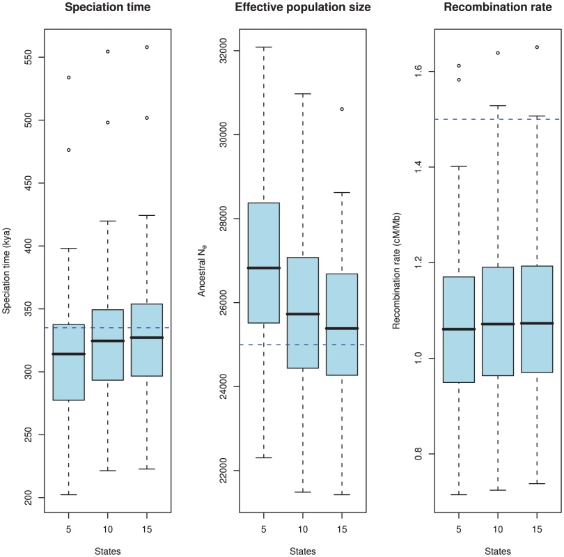
The boxplots show the estimated parameters (divergence time, ancestral effective population size, and recombination rate) for 100 simulated data sets. The true value is showed as the blue dashed line. The number of states in the HMM, i.e. the number of coalescence time intervals used for the estimation takes the values 5, 10 and 15. There is a clear bias in the estimates where we tend to underestimate the divergence time and overestimate the effective population size. This bias is caused by the discretisation of continuous coalescence times into fixed intervals, and the bias is reduced as the number of states (i.e. intervals) increases. The recombination rate is under-estimated, which is a consequence of the Markov assumption. As is evident from the figure, there is a bias in the estimates: we tend to underestimate the split time and at the same time overestimate the ancestral population size. Similar biases were observed in our previous model based on incomplete lineage sorting rather than changes in divergence time [12]. Both biases are probably caused by the same modeling artifact: For the model to fit the data, it must predict a sequence divergence close to the observed value, so if the split time is decreased, the effective population size must increase to reach the same average divergence, and vice versa. The recombination rate is somewhat underestimated for all runs.
To elucidate the source of the biases we did an extensive set of simulations with different subsets of our model assumptions met, see Protocol S1. Simulating directly from the HMM, where all model assumptions are met, we find no bias in any of the three parameters. Simulating from the coalescent process with recombination but discretizing time to the mean of each time interval, we only see the bias on the recombination rate but no longer the biases on divergence time and effective population size. Simulating from a coalescent process with the Markov assumption but continuous time intervals [20] we see the bias on the recombination rate disappear.
Based on the simulation study, we believe that the bias in the recombination rate is caused by the Markov assumption along the alignment, and that the bias in divergence time and effective population size is caused by the discretization of coalescence times into fixed intervals, and we observe that the bias indeed decreases as we increase the number of intervals and thus more accurately capture the true distribution.
With 10 states, the biases on split time and effective population size are reduced compared to 5 states, and the gain of adding an additional 5 states is minor in comparison. For computational efficiency (since the algorithm scales quadratically in the number of states), we used 10 states in the orangutan analysis.
Analysis of the orangutan sub-species
We aligned the two orangutan genomes and divided the alignment into 2,689 1 Mbp segments, obtaining independent maximum likelihood estimates of the divergence time, effective population size of the ancestral species, and recombination rate for each segment. The estimates are based on a mutation rate of per year and a generation time of 20 years, giving substitutions per generation. For the effective population size of the two sub-species we used estimates from Becquet and Przeworski [3]: for Bornean orangutans and for Sumatran orangutans. The genome-wide estimates are summarized in Table 1.
Tab. 1. Genome-wide parameter estimates. 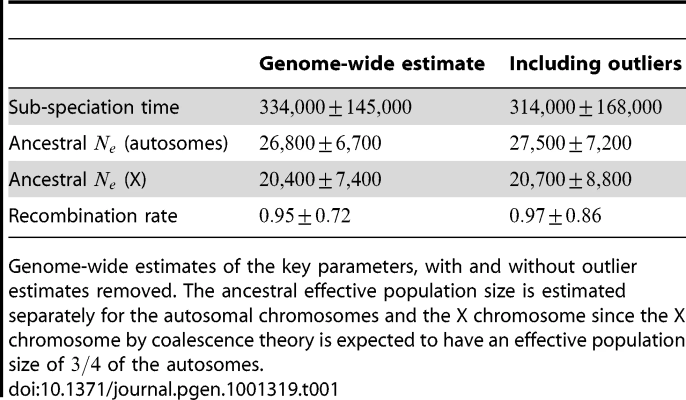
Genome-wide estimates of the key parameters, with and without outlier estimates removed. The ancestral effective population size is estimated separately for the autosomal chromosomes and the X chromosome since the X chromosome by coalescence theory is expected to have an effective population size of of the autosomes. After inferring parameters for each segment we removed outlier segments where the inferred divergence time was below 5 thousand years or above 1 million years; the effective population size was below 5,000 or above 100,000; and where the recombination rate was below 0.1 or above 10. In total 203 segments were removed, leaving 2486. Removing these outliers had very little effect on the genome-wide estimates (see Table 1).
Divergence time
We obtained an independent estimate of the sub-species divergence time for each of the 1 Mbp segments. Figure 9 shows the distribution of these estimates for each chromosome and Supplemental Figure 3 of Protocol S1 shows the distribution for the entire genome. In general, the estimates on the different chromosomes are consistent. For chromosome 21, the genomic mean estimate is not within the 50% confidence interval (the blue box in the box-plot), but it is within the 95% confidence interval. The genome-wide average is thousand years ago (kya).
Fig. 9. Distribution of sub-speciation time estimates for each chromosome. 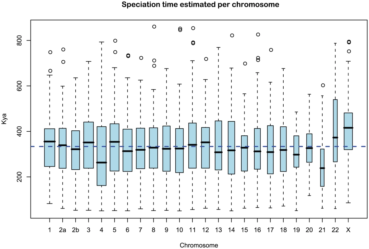
The box plot shows the distribution of the estimated sub-speciation time on each chromosome. The dashed line shows the genome-wide average. In general, the estimates are reasonably consistent between the chromosomes, although chromosome 21 has a slightly smaller value. Ancestral effective population sizes
Figure 10 and Supplemental Figure 4 of Protocol S1 show the estimates of the ancestral effective population size for each chromosome and for the entire genome, respectively. Since the X chromosome is expected to have an effective population size of of that of the autosomes, we estimate the genome-wide effective population size from the autosomes only and obtain . The estimate for the X chromosome is , close to the expected of the estimate from the autosomes.
Fig. 10. Distribution of effective population size estimates for each chromosome. 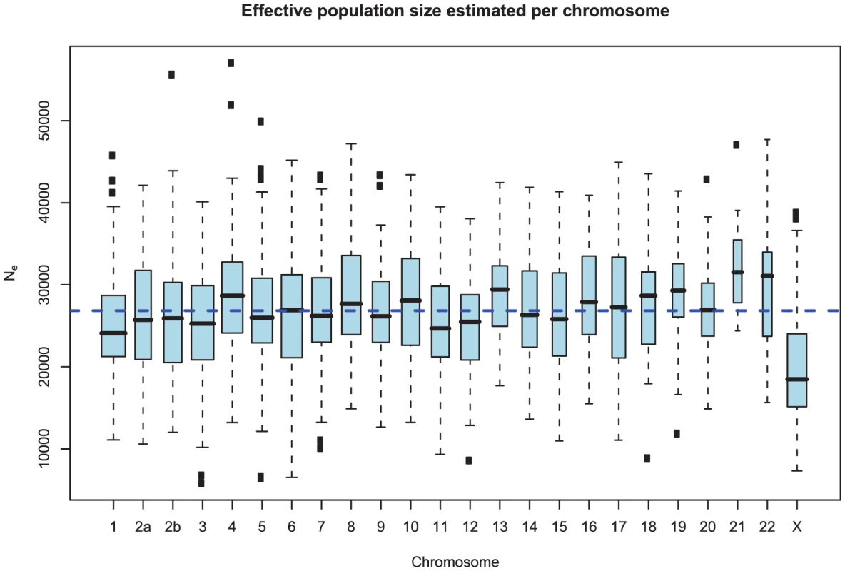
The box plot shows the distribution of the estimated ancestral effective population on each chromosome. The dashed line shows the genome-wide average. In general, the estimates are reasonably consistent between the chromosomes, with one exception being chromosome 21. Chromosome X is within the expected range of of the autosomal chromosomes. As for the estimates of the divergence time, the estimates are consistent between chromosomes. Again, the genomic mean is not contained within the 50% confidence interval, but is within the 95% interval. This is likely to be related to the observation for the divergence time estimates in Figure 9, as the parameter for divergence time and for ancestral population size are confounded. In general, if we underestimate the divergence time we overestimate the effective population size, leaving the average divergence less affected.
Recombination rate
Figure 11 and Supplemental Figure 5 of Protocol S1 show the estimates of the recombination rate for each chromosome and for the entire genome, respectively. We estimate the genome-wide recombination rate to be cM/Mb. The absolute value should be interpreted with caution, however, since we know from the simulation study that the recombination rate is likely to be under-estimated. The estimated recombination rate correlates positively with the equilibrium GC content, as estimated from the substitution model (Figure 12) as has also been observed for human polymorphism data.
Fig. 11. Distribution of recombination rate estimates for each chromosome. 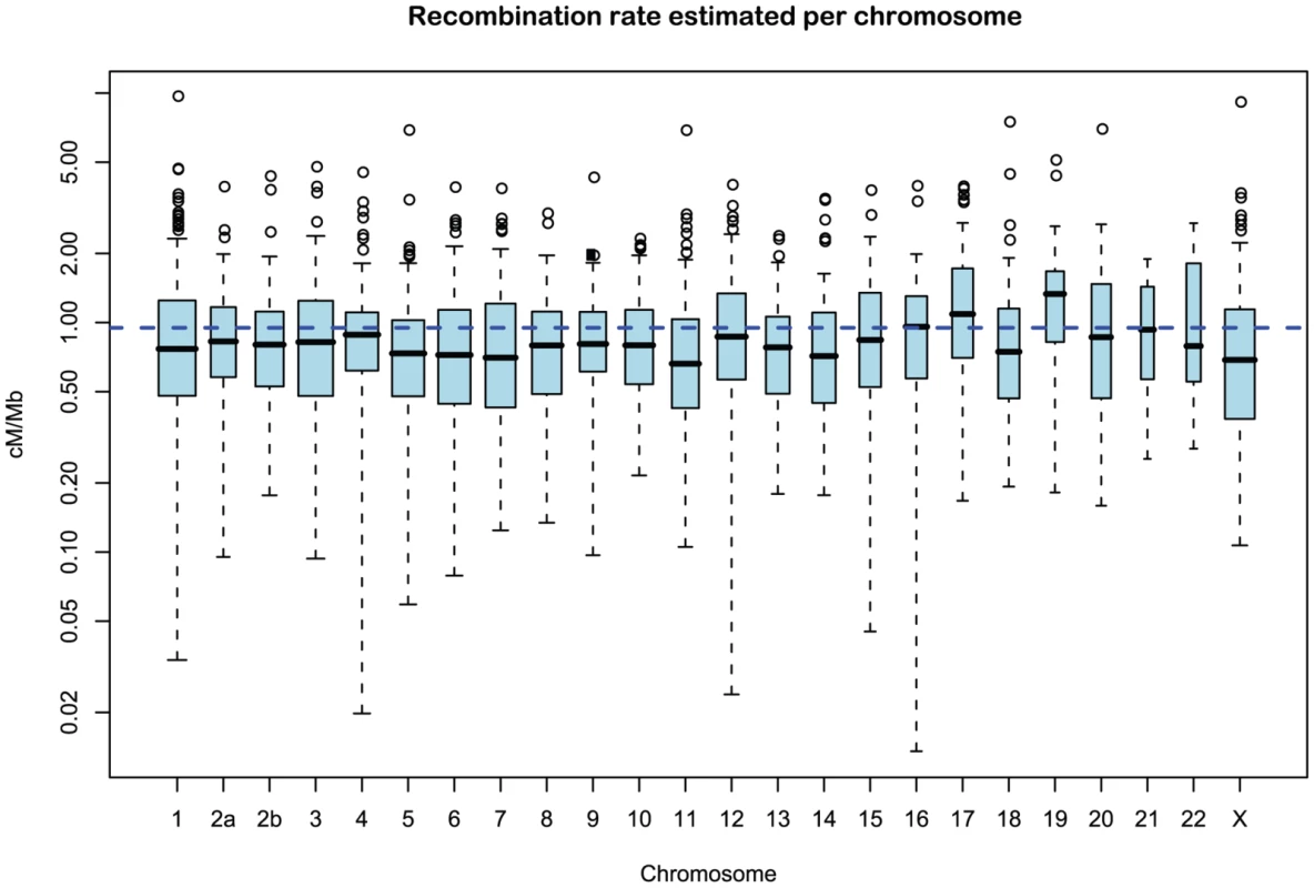
The box plot shows the distribution of the estimated recombination rate for each chromosome. The dashed line shows the genome-wide average. Fig. 12. The correlation between GC content and inferred recombination rate. 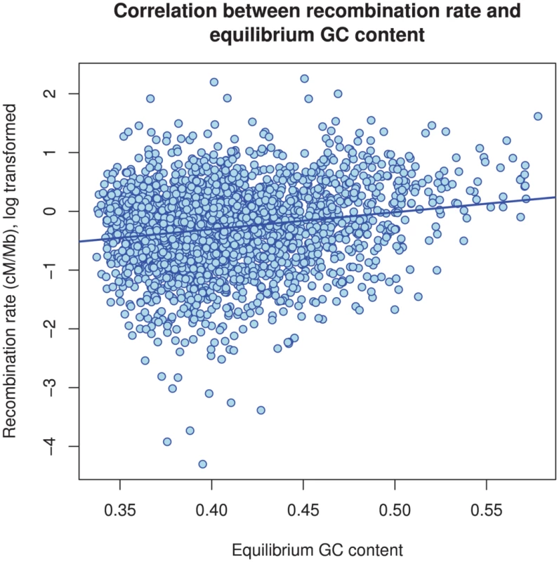
There is a significant positive correlation between recombination rate and (equilibrium) GC content (). Differences between chromosomes
Figure 13 shows the average estimates of the key parameters for each chromosome as a function of the chromosome size (measured as the number of segments analyzed). We find no correlation between the divergence time and the chromosome size, but a negative correlation between inferred recombination rate and size. This suggests higher recombination rate per base pair at small chromosomes as is also observed in the human genome. Interestingly, the effective population size is also significantly higher on the smaller and more recombining chromosomes.
Fig. 13. The correlation of inferred parameters with chromosome size. 
A) There is no correlation between the estimated sub-speciation time and chromosome size. B) A negative correlation between chromosome size and estimated recombination rate (). C) A negative correlation between chromosome size and inferred effective population size (). The X chromosome was removed from the regression of effective population size. Robustness of the results
The estimates are conditional on the parameters we have kept fixed in the model: the mutation rate, the generation time, the effective population size of the two present day populations, and the number of hidden states.
Since coalescence time is scaled in time units of generations and emission probabilities are given by the mutation (substitution) rate times the divergence time, changing either the assumed generation time (20 years per generation) or the assumed mutation rate ( mutations per generation) will change the estimated divergence time linearly: since time in the model is measured in generations, halving the generation time would halve the divergence time when measured in years. Similarly, assuming that the mutation rate is twice as high, the inferred divergence time would be half as long ago.
Less obvious is the dependency on the present day effective population sizes and the number of states in the HMM. To test this we varied the fixed effective population sizes by a factor of 10 in both direction and alternatively tried constraining the three effective population sizes in the model to be equal. We found the resulting changes in the estimates to be insignificant. Similarly, changing the number of states did not change the estimated parameters significantly. For details, see Supplemental Section 2.3 of Protocol S1.
Discussion
We present a new model for the analysis of two genomes from diverged populations or closely related species, with the aim of estimating divergence time, the effective population size of the ancestral population, and the recombination rate.
Simulation results show that the model infers the key parameters without much bias when the number of coalescent states is sufficiently high (we recommend at least 10 states). The estimates are not much affected by assumptions of the effective size of the present day populations, which implies that the model can be used for analysis of population pairs where only the order of magnitude of these quantities are known. That the model produces consistent results may seem surprising since the model is essentially only modeling what happens from one nucleotide to the next and not any higher order correlations. This is very fortunate since it is the Markov property that enables calculations to be sufficiently efficient for genome-wide analysis.
Consequences of migration
The present model assumes a simple population split or an allopatric speciation. To test the consequences of this assumption, we simulated data sets where a single population first splits into two populations with some gene-flow between the populations, and some time later the gene-flow stops (see Protocol S1).
In this setting, the divergence time we infer is between the first and the second time point; usually closer to the time point where gene-flow stopped unless the migration rate is very low. This makes sense since the split time modeled in our approach is exactly the termination of genetic flow between the two lineages, and not the introduction of structure in the ancestral population.
Only the split time parameter seemed to be affected to a larger extend by gene-flow. The effective population size was slightly over-estimated when gene-flow is present, more so if the time interval and migration rate are large, but the effect is small relative to the variance on the estimates. The recombination rate is estimated to be somewhat higher with gene-flow, again higher when the time interval and mutation rate are high, but is still biased and estimated below the simulated rate.
Consequences of unknown phase
Our model assumes that the input data is an alignment of two haploid genomes where neighboring nucleotides are linked on the same chromosome, but in the analysis we use reference genome sequences that each are a mosaic of at least two haploid genomes.
A consequence of this is that the assumption we make about the two neighbouring nucleotides being linked at the present day is incorrect (see also Figure 3). If the recombination/coalescence process is close to equilibrium, assumptions about the starting point are irrelevant, but with an effective size on the order of and speciation time of years we do not expect that the process has reached equilibrium, and thus the unknown phase could potentially affect our estimates.
However, varying the present day effective population size parameters an order of magnitude in either direction (see Supplemental Figure 10 of Protocol S1) gave essentially identical results for the parameter estimates, so we trust that treating the reference genome sequences as if they were present day haploid genomes is not a source of bias.
Orangutan analysis
Our estimates on effective sizes and speciation time are in close agreement with an analysis based on SNP frequencies from full genome sequencing of five individuals of each of the subspecies (included in the Orangutan Genome paper [17]). Results disagree with Bequet and Przeworski [3] who reported a split time of 1.4 million years and an ancestral effective size of (C.I. ). They used MIMAR to infer parameters. The same authors have shown that MIMAR is quite sensitive to population structure in the ancestral species. Furthermore, their parameters correspond to an average divergence time of the two subspecies of 1.4 my plus years. If we assume years per generation then years will be million years and a total divergence of million years. This does not seem to be supported by the average divergence of the subspecies which is estimated close to million years [17], therefore we believe there must be a bias in the estimates by Becquet and Przeworski.
The X chromosome is found to have an effective population size almost exactly 3/4 of the autosome average. This suggests that selection has not affected the X chromosomes in a different way than the autosomes between the two orangutan sub-species, in contrast to the reports from the human-chimpanzee analyses [2], [5].
Further validation that the model contains information in addition to a simple sliding window analysis of divergence is provided by the observation that small chromosomes are found to have higher recombination rate estimates. This is in line with genetic maps of the human genome (and other genomes) and is believed to be a consequence of the necessity of a least one crossover event per chromosomes for proper segregation in meiosis. The observed correlation between GC content and recombination rate was also expected from similar correlations in other species.
This leads us to the negative correlation between effective size and chromosome size observed. Why should smaller chromosomes have higher effective population sizes? We suggest that this is due to their higher average recombination rates, which reduces the effects of background selection and hitch-hiking, both of which tend to increase coalescence rates and thus decrease estimates of effective population size. If this suggestion is true, it shows a large role for selection on determining effective population size, in accordance with the large role proposed in the recent study by McVicker et al. [21].
Future prospects
The simple model presented here can be extended to more populations by extending the number of transition states. It may therefore also be combined with the HMM models that analyse incomplete lineage sorting [5], [12]. This would allow better consideration of substitution rate heterogeneity along the genome.
The limiting factor in a straightforward extension of the method to more genomes is the state explosion in the CTMC as more and more combinations of sequences must be considered. While the single sequence CTMC has two states and two non-zero transition-rates, and the two sequence CTMC has 15 states and 44 non-zero transition-rates, three sequences would have 203 states and 1,118 non-zero rates and four sequences would have 4,140 states and 35,446 non-zero rates, making the approach impractical for more than a few genomes. We do, however, believe that it is possible to extend the method to three genomes, combining the CTMC approach presented here with the incomplete lineage sorting model used in our previous CoalHMMs [5], [12].
We also believe that the approach of computing transition probabilities based on coalescence calculations on two neighboring nucleotides can be extended to more complex scenarios such as gene flow following the population split or (sub-)speciation. Since we are explicitly modeling the coalescence process for two nucleotides, the framework generalizes to essentially all scenarios that can be modeled with the coalescence process, without the need for approximating these.
Posterior decoding of the states is also a promising avenue for inferring changes in population size over time in the ancestral population [1], [5], [12], [21]. Likewise, posterior decoding might be a powerful approach to the detection of selective sweeps in the ancestral population as long segments with the same divergence time.
A simulation study is presently exploring this opportunity of ancestral demographics and we believe that the present model is ideally suited for this.
Materials and Methods
The orangutan sub-species alignment
The pairwise sub-species alignment was created from a set of 36 bp paired-end Illumina reads from a single Bornean Orangutan individual, which were mapped to the reference Sumatran genome assembly, and sorted by genomic position. Only reads that passed a stringent set of filters were used to create the Bornean sequence and alignment. For single-end reads, the criteria were: mapping quality at least 10 (Phred scale), likelihood score at most 90 (Phred), at most 3 variants with respect to the reference, and at most a single gap. for paired-end reads, the criteria were identical, except that a likelihood score of up to 140 was accepted, and in addition the distance between the mate pairs was required not to exceed 700.
A pileup was next created from those reads passing filters. Variants (both SNPs and indels) were called based on a simple majority-vote scheme, weighted by the qualities of the bases. Bases that were within 5 bp of either end of a read, were not taken into account, because uncalled indel variants cause systematic apparent base changes that otherwise lead to false SNP calls. The voting scheme consisted of adding together the base qualities of the eligible bases for each supported variant, where the reference base was assigned a prior of 30 (on a Phred scale). An indel was called if it was seen at least twice, with at least one being called at a minimum distance of at least 10 bases from either end of the read, not counting uncalled bases, and bases with quality score 0. A variant was called only when the coverage at the locus (after filtering, but not including the 5 bp read fringe filter) was between 3 and 20 reads.
The algorithm produced a pairwise alignment in .axt format directly from the resulting stream of indel and SNP calls. Regions where insufficient read coverage was available to call variants were annotated in lower case, and not considered in the subsequent analysis. It is important to note that regions of possible paralogy, such as recent segmental duplications, would cause low mapping qualities in the reads derived from them. Possible paralogous regions therefore do not contribute towards the subsequent analyses.
The coalescent hidden Markov model
To estimate population genetic parameters we exploit how the underlying coalescence process causes the divergence time of the two genomes to vary along the alignment. We split the possible divergence times into discrete time intervals and use these as states in a hidden Markov model, where transition and emission probabilities are derived from parameters in the coalescent process. Transition probabilities are modelled using two-nucleotide continuous time Markov chains; the emission probabilities are modelled as continuous time Markov chain substitution models in the usual way.
Modelling sequence divergence using two-nucleotide continuous time Markov chains
We approximate the distribution of segment lengths in time using two-nucleotide continuous time Markov chains (CTMCs), where left and right nucleotides can be linked or unlinked, and where left/right nucleotides can be coalesced (i.e. have found their most recent common ancestor) or not.
We model the evolution of a sequence in a single population as a two state CTMC. State 1 corresponds to the two nucleotides being linked and state 2 corresponds to the two nucleotides being unlinked (see Figure 2). Linked nucleotides become unlinked with rate and unlinked nucleotides become linked with rate . Letting be the per generation per nucleotide recombination rate we have . Furthermore we have , where is the effective population size for the reference population. The rate matrix for a single population is thus(1)and the state of the two nucleotides at time is determined by the probability matrix . If the initial nucleotides are linked (in state 1) then they are also linked at time with probability and unlinked with probability .
The ancestral population is modelled using a CTMC where nucleotides can have coalesced or not and where left and right nucleotides can be linked or not . The state space is summarized in Figure 4, and the corresponding rate matrix is given by(2)The size of the state space is 15 and the rate matrix is naturally structured in four different classes. The first class (with seven states) are the states where coalescence of left or right nucleotides has not yet occurred. The second class of states (with three states) consists of the states where coalescence of the left nucleotides has occurred, and the third class of states is where coalescence of right nucleotides has occurred. Finally, the last class of states is the states where coalescence of both right and left nucleotides has occurred. We call the four classes of states , , and , where and stands for right and left, respectively, stands for beginning, and for ending. Note that the chain must start in the beginning states 1–7. Also note that states 1–10 are transient while state 14 and 15 are persistent.
In Figure 14 we show the isolation model of the two populations. Back in time, the two populations are first isolated and behave according to the single sequence system. The two populations have effective population sizes and , respectively, with corresponding rate matrices and .
Fig. 14. Isolation model. 
Left: Parameters of the model; we use the ancestral population as the reference population. Right: Rate matrices for the single sequence systems and (ancestral) two-sequence system. At the population divergence time the two sequences system is entered. The two sequences system is entered in state 1-4 depending on the states of each of the two single sequence systems. Let denote the initial distribution of the two species system. The two sequences system has effective population size and the corresponding rate matrix is .
Transition probabilities in the hidden Markov model
The states of the hidden Markov model (HMM) correspond to different coalescence times. We use time intervals, with break points . State then corresponds to coalescence in the interval , where . The CTMC allows us to determine the transition probabilities of the HMM.
The distribution of the CTMC states, when entering HMM state (at time ) is given by where . Let be the equilibrium distribution for the CTMC.
Let denote the probability that the left nucleotide in the two sequences CTMC coalesce in HMM state , i.e. in the time interval and that the right nucleotide coalesce in state , i.e. in the time interval . Let denote the (marginal) probability that the left nucleotide coalesce in state . The transition probability from state to state in the HMM is then given by(3)
The marginal coalescence times are given by the exponential distribution with rate ; where .
Let denote the two-nucleotide state of the CTMC at time and let denote the probability distribution of the CTMC at time . If we obtain the joint probability fromand if we get
In the case similar calculations apply, but due to symmetries in the process within the ancestral species, also applies.
Calculated this way, the transition probabilities are exact according to the coalescence process with recombination and, unlike previous CoalHMMs, not an approximation to the process. While the CoalHMM we have developed here is still an approximation to the full coalescent process, due to the Markov assumption and the way we define emission probabilities, this is still an important improvement over previous CoalHMMs.
The equations above are valid for any choice of time intervals as the states in the CTMC. For the analysis of the orangutan sub-species we chose a simple strategy of choosing the intervals to be equi-probable, i.e. such that the stationary state probability for the HMM puts equal probability on all states.
Emission probabilities
Emission probabilities are the probabilities that a given pair of nucleotides are separated by a given time. A CTMC of nucleotide change is assumed, following work by Felsenstein [22], and the probabilities are obtained by computing the matrix exponential of the model generator, multiplied by the divergence time. The large amount of data available here allowed us to use parameter rich substitution models like the General Time Reversible model. This model includes as parameters the equilibrium GC content and distinct transition and transvertion rates. When calculating the emission probability for a state, we use the mean time point in the corresponding time interval.
Estimating parameters
For each segment, the parameters estimated was the maximum likelihood parameters. A modified Newton-Raphson algorithm was used to find the maximum of the likelihood function. The first - and second-order derivatives with respect to the parameters were computed numerically using the three-points method.
Supporting Information
Zdroje
1. SiepelA
2009 Perspective: Phylogenomics of primates and their ancestral populations. In review
2. PattersonN
RichterDJ
GnerreS
LanderES
ReichD
2006 Genetic evidence for complex speciation of humans and chimpanzees. Nature 441 1103 1108
3. BecquetC
PrzeworskiM
2007 A new approach to estimate parameters of speciation models with application to apes. Genome Res 17 1505 1519
4. RannalaB
YangZ
2003 Bayes estimation of species divergence times and ancestral population sizes using dna sequences from multiple loci. Genetics 164 1645 1656
5. HobolthA
ChristensenOF
MailundT
SchierupMH
2007 Genomic relationships and speciation times of human, chimpanzee, and gorilla inferred from a coalescent hidden markov model. PLoS Genet 3 e7 doi:10.1371/journal.pgen.0030007
6. BurgessR
YangZ
2008 Estimation of hominoid ancestral population sizes under bayesian coalescent models incorporating mutation rate variation and sequencing errors. Mol Biol Evol 25 1979 1994
7. HeinJ
SchierupMH
WiufC
2005 Gene genealogies, variation and evolution: A primer in coalescent theory Oxford university press
8. TakahataN
1986 An attempt to estimate the effective size of the ancestral species common to 2 extant species from which homologous genes are sequenced. Genetical Research 48 187 190
9. TakahataN
1989 Gene genealogy in 3 related populations - consistency probability between gene and population trees. Genetics 122 957 966
10. YangZH
1997 On the estimation of ancestral population sizes of modern humans. Genetical Research 69 111 116
11. WallJD
2003 Estimating ancestral population sizes and divergence times. Genetics 163 395 404
12. DutheilJY
GanapathyG
HobolthA
MailundT
UyenoyamaMK
2009 Ancestral population genomics: The coalescent hidden markov model approach. Genetics 183 259 274
13. HeyJ
NielsenR
2004 Multilocus methods for estimating population sizes, migration rates and divergence time, with applications to the divergence of drosophila pseudoobscura and d. persimilis. Genetics 167 747 760
14. HudsonRR
1983 Properties of a neutral allele model with intragenic recombination. Theor Popul Biol 23 183 201
15. WiufC
HeinJ
1997 On the number of ancestors to a DNA sequence. Genetics 147 1459 1468
16. WiufC
HeinJ
1999 The ancestry of a sample of sequences subject to recombination. Genetics 151 1217 1228
17. LockeD
Unveiling the ancient diversity and slow evolution of the orangutan genome. In progress
18. WiufC
HeinJ
1999 Recombination as a point process along sequences. Theor Popul Biol 55 248 259
19. MarjoramP
WallJ
2006 Fast ‘coalescent’ simulations. BMC Genetics 7 16
20. ChenGK
MarjoramP
WallJD
2009 Fast and exible simulation of DNA sequence data. Genome Res 19 136 42
21. McVickerG
GordonD
DavisC
GreenP
2009 Widespread genomic signatures of natural selection in hominid evolution. PLoS Genet 5 e1000471 doi:10.1371/journal.pgen.1000471
22. FelsensteinJ
1981 Evolutionary trees from dna sequences: a maximum likelihood approach. J Mol Evol 17 368 76
Štítky
Genetika Reprodukční medicína
Článek Genetic Regulation by NLA and MicroRNA827 for Maintaining Nitrate-Dependent Phosphate Homeostasis inČlánek c-di-GMP Turn-Over in Is Controlled by a Plethora of Diguanylate Cyclases and PhosphodiesterasesČlánek Viral Genome Segmentation Can Result from a Trade-Off between Genetic Content and Particle Stability
Článek vyšel v časopisePLOS Genetics
Nejčtenější tento týden
2011 Číslo 3- Akutní intermitentní porfyrie
- Růst a vývoj dětí narozených pomocí IVF
- Vliv melatoninu a cirkadiálního rytmu na ženskou reprodukci
- Délka menstruačního cyklu jako marker ženské plodnosti
- Farmakogenetické testování pomáhá předcházet nežádoucím efektům léčiv
-
Všechny články tohoto čísla
- Whole-Exome Re-Sequencing in a Family Quartet Identifies Mutations As the Cause of a Novel Skeletal Dysplasia
- Origin-Dependent Inverted-Repeat Amplification: A Replication-Based Model for Generating Palindromic Amplicons
- Testing for an Unusual Distribution of Rare Variants
- Limited dCTP Availability Accounts for Mitochondrial DNA Depletion in Mitochondrial Neurogastrointestinal Encephalomyopathy (MNGIE)
- FUS Transgenic Rats Develop the Phenotypes of Amyotrophic Lateral Sclerosis and Frontotemporal Lobar Degeneration
- Repeat Associated Non-ATG Translation Initiation: One DNA, Two Transcripts, Seven Reading Frames, Potentially Nine Toxic Entities!
- Initial Mutations Direct Alternative Pathways of Protein Evolution
- Dopamine Signalling in Mushroom Bodies Regulates Temperature-Preference Behaviour in
- Sensing of Replication Stress and Mec1 Activation Act through Two Independent Pathways Involving the 9-1-1 Complex and DNA Polymerase ε
- Genetic Regulation by NLA and MicroRNA827 for Maintaining Nitrate-Dependent Phosphate Homeostasis in
- Identification of a Novel Type of Spacer Element Required for Imprinting in Fission Yeast
- Chiasmata Promote Monopolar Attachment of Sister Chromatids and Their Co-Segregation toward the Proper Pole during Meiosis I
- Global Analysis of the Relationship between JIL-1 Kinase and Transcription
- H3K9me2/3 Binding of the MBT Domain Protein LIN-61 Is Essential for Vulva Development
- REVEILLE8 and PSEUDO-REPONSE REGULATOR5 Form a Negative Feedback Loop within the Arabidopsis Circadian Clock
- A Novel Unstable Duplication Upstream of Predisposes to a Breed-Defining Skin Phenotype and a Periodic Fever Syndrome in Chinese Shar-Pei Dogs
- Polycomb Repressive Complex 2 Controls the Embryo-to-Seedling Phase Transition
- A Role for Set1/MLL-Related Components in Epigenetic Regulation of the Germ Line
- Genome-Wide Association Analysis Identifies Variants Associated with Nonalcoholic Fatty Liver Disease That Have Distinct Effects on Metabolic Traits
- A Genome-Wide Association Study of Upper Aerodigestive Tract Cancers Conducted within the INHANCE Consortium
- Ancestral Mutation in Telomerase Causes Defects in Repeat Addition Processivity and Manifests As Familial Pulmonary Fibrosis
- Ultra-Deep Sequencing of Mouse Mitochondrial DNA: Mutational Patterns and Their Origins
- Phenotype Restricted Genome-Wide Association Study Using a Gene-Centric Approach Identifies Three Low-Risk Neuroblastoma Susceptibility Loci
- The Toll-Like Receptor Gene Family Is Integrated into Human DNA Damage and p53 Networks
- Polycomb Targets Seek Closest Neighbours
- Widespread Hypomethylation Occurs Early and Synergizes with Gene Amplification during Esophageal Carcinogenesis
- c-di-GMP Turn-Over in Is Controlled by a Plethora of Diguanylate Cyclases and Phosphodiesterases
- Estimating Divergence Time and Ancestral Effective Population Size of Bornean and Sumatran Orangutan Subspecies Using a Coalescent Hidden Markov Model
- Rif1 Supports the Function of the CST Complex in Yeast Telomere Capping
- A Tradeoff Drives the Evolution of Reduced Metal Resistance in Natural Populations of Yeast
- Quantifying the Underestimation of Relative Risks from Genome-Wide Association Studies
- Population-Based Resequencing of Experimentally Evolved Populations Reveals the Genetic Basis of Body Size Variation in
- Triplet Repeat–Derived siRNAs Enhance RNA–Mediated Toxicity in a Drosophila Model for Myotonic Dystrophy
- The FUN30 Chromatin Remodeler, Fft3, Protects Centromeric and Subtelomeric Domains from Euchromatin Formation
- Viral Genome Segmentation Can Result from a Trade-Off between Genetic Content and Particle Stability
- Environmental Sex Determination in the Branchiopod Crustacean : Deep Conservation of a Gene in the Sex-Determining Pathway
- Systematic Detection of Polygenic Regulatory Evolution
- The SUMO Isopeptidase Ulp2p Is Required to Prevent Recombination-Induced Chromosome Segregation Lethality following DNA Replication Stress
- Uncoupling Antisense-Mediated Silencing and DNA Methylation in the Imprinted Cluster
- Role of the Drosophila Non-Visual ß-Arrestin Kurtz in Hedgehog Signalling
- Differential Genetic Associations for Systemic Lupus Erythematosus Based on Anti–dsDNA Autoantibody Production
- COMPASS-Like Complexes Mediate Histone H3 Lysine-4 Trimethylation to Control Floral Transition and Plant Development
- H3 Lysine 4 Is Acetylated at Active Gene Promoters and Is Regulated by H3 Lysine 4 Methylation
- Diverse Roles and Interactions of the SWI/SNF Chromatin Remodeling Complex Revealed Using Global Approaches
- A Bow-Tie Genetic Architecture for Morphogenesis Suggested by a Genome-Wide RNAi Screen in
- Roles of () in Oocyte Nuclear Architecture, Gametogenesis, Gonad Tumors, and Genome Stability in Zebrafish
- A Molecular Phylogeny of Living Primates
- Roles of the Espin Actin-Bundling Proteins in the Morphogenesis and Stabilization of Hair Cell Stereocilia Revealed in CBA/CaJ Congenic Jerker Mice
- A Cholinergic-Regulated Circuit Coordinates the Maintenance and Bi-Stable States of a Sensory-Motor Behavior during Male Copulation
- PLOS Genetics
- Archiv čísel
- Aktuální číslo
- Informace o časopisu
Nejčtenější v tomto čísle- Whole-Exome Re-Sequencing in a Family Quartet Identifies Mutations As the Cause of a Novel Skeletal Dysplasia
- Origin-Dependent Inverted-Repeat Amplification: A Replication-Based Model for Generating Palindromic Amplicons
- FUS Transgenic Rats Develop the Phenotypes of Amyotrophic Lateral Sclerosis and Frontotemporal Lobar Degeneration
- Limited dCTP Availability Accounts for Mitochondrial DNA Depletion in Mitochondrial Neurogastrointestinal Encephalomyopathy (MNGIE)
Kurzy
Zvyšte si kvalifikaci online z pohodlí domova
Autoři: prof. MUDr. Vladimír Palička, CSc., Dr.h.c., doc. MUDr. Václav Vyskočil, Ph.D., MUDr. Petr Kasalický, CSc., MUDr. Jan Rosa, Ing. Pavel Havlík, Ing. Jan Adam, Hana Hejnová, DiS., Jana Křenková
Autoři: MUDr. Irena Krčmová, CSc.
Autoři: MDDr. Eleonóra Ivančová, PhD., MHA
Autoři: prof. MUDr. Eva Kubala Havrdová, DrSc.
Všechny kurzyPřihlášení#ADS_BOTTOM_SCRIPTS#Zapomenuté hesloZadejte e-mailovou adresu, se kterou jste vytvářel(a) účet, budou Vám na ni zaslány informace k nastavení nového hesla.
- Vzdělávání


