-
Články
- Vzdělávání
- Časopisy
Top články
Nové číslo
- Témata
- Kongresy
- Videa
- Podcasty
Nové podcasty
Reklama- Kariéra
Doporučené pozice
Reklama- Praxe
Incorporating Biological Pathways via a Markov Random Field Model in Genome-Wide Association Studies
Genome-wide association studies (GWAS) examine a large number of markers across the genome to identify associations between genetic variants and disease. Most published studies examine only single markers, which may be less informative than considering multiple markers and multiple genes jointly because genes may interact with each other to affect disease risk. Much knowledge has been accumulated in the literature on biological pathways and interactions. It is conceivable that appropriate incorporation of such prior knowledge may improve the likelihood of making genuine discoveries. Although a number of methods have been developed recently to prioritize genes using prior biological knowledge, such as pathways, most methods treat genes in a specific pathway as an exchangeable set without considering the topological structure of a pathway. However, how genes are related with each other in a pathway may be very informative to identify association signals. To make use of the connectivity information among genes in a pathway in GWAS analysis, we propose a Markov Random Field (MRF) model to incorporate pathway topology for association analysis. We show that the conditional distribution of our MRF model takes on a simple logistic regression form, and we propose an iterated conditional modes algorithm as well as a decision theoretic approach for statistical inference of each gene's association with disease. Simulation studies show that our proposed framework is more effective to identify genes associated with disease than a single gene–based method. We also illustrate the usefulness of our approach through its applications to a real data example.
Published in the journal: . PLoS Genet 7(4): e32767. doi:10.1371/journal.pgen.1001353
Category: Research Article
doi: https://doi.org/10.1371/journal.pgen.1001353Summary
Genome-wide association studies (GWAS) examine a large number of markers across the genome to identify associations between genetic variants and disease. Most published studies examine only single markers, which may be less informative than considering multiple markers and multiple genes jointly because genes may interact with each other to affect disease risk. Much knowledge has been accumulated in the literature on biological pathways and interactions. It is conceivable that appropriate incorporation of such prior knowledge may improve the likelihood of making genuine discoveries. Although a number of methods have been developed recently to prioritize genes using prior biological knowledge, such as pathways, most methods treat genes in a specific pathway as an exchangeable set without considering the topological structure of a pathway. However, how genes are related with each other in a pathway may be very informative to identify association signals. To make use of the connectivity information among genes in a pathway in GWAS analysis, we propose a Markov Random Field (MRF) model to incorporate pathway topology for association analysis. We show that the conditional distribution of our MRF model takes on a simple logistic regression form, and we propose an iterated conditional modes algorithm as well as a decision theoretic approach for statistical inference of each gene's association with disease. Simulation studies show that our proposed framework is more effective to identify genes associated with disease than a single gene–based method. We also illustrate the usefulness of our approach through its applications to a real data example.
Introduction
In genome-wide association studies (GWAS) researchers examine a large number of markers across the genome in many individuals to identify associations between genetic variants and disease, or to prioritize markers for follow up studies. However, most of the times the signals from individual markers are weak and the sample size is not large enough to have adequate power for true discoveries, especially when the minor allele frequency is low. Various approaches have been developed to increase statistical power, including aggregating multiple markers from the same gene or in the same haplotype block region and incorporating information from other sources into the GWAS analysis. It has been found that the gene level analysis has the ability to identify new associations in addition to those identified using individual Single Nucleotide Polymorphisms (SNPs) [1], [2]. Gene-based analyses include those using the most significant SNP within and near a gene [1]; combination statistics (Fisher, Sidat, and Simes) from all individual markers [2]; Principal Component Analysis (PCA) regressions [3] and the sparse partial least squares regressions [4]. To incorporate prior biological knowledge, one information rich resource is biological pathways. It is believed that genes interact with each other in biological processes, and it is conceivable that they may jointly affect the risk of a complex disease. There exist an abundance of databases containing known gene pathways and protein-protein interactions, such as KEGG, BioCarta, GenMAPP, and HPRD. A number of gene prioritization methods incorporating prior biological knowledge have been developed for GWAS. Some examples include Prioritizer [5], Endeavour [6], CGI [7], CANDID [8], GeneWanderer [9], CIPHER [10], GIN [11], and the pathway based gene set enrichment approach [1]. These methods have shown that incorporating prior biological information in GWAS is useful. However, they do not consider functional relationships among genes. The general input of these approaches is a list of genes as a set, in which genes are treated as exchangeable without taking into account the regulatory relationships among them. As a result, information from the pathway topology and interactions among genes is usually ignored. However, how genes are functionally related to each other in a pathway may be very informative for GWAS analysis and such information can be utilized to increase the power of detecting real associations. When associations have been firmly established for some genes either through GWAS or prior candidate gene-based studies, we can take advantage of this knowledge to examine other genes related to these known genes through the same pathways they all participate in.
In this paper we propose a Markov Random Field (MRF) model to incorporate biological pathway information in GWAS. MRF has been considered by several authors to combine data from different sources in genomics studies, e.g., a spatial normal mixture model [12] for gene expression and CHIP-chip data, a Gamma-Gamma model and MRF for mRNA microarray data [13], and prioritizing genes by combining gene expression and protein interaction data [7]. However, little has been done in the context for GWAS, with the exception of Li et al. [14] who proposed a hidden MRF for GWAS. But their method is developed in the context of jointly analyzing markers in linkage disequilibrium.
We first present a motivating example from a GWAS of Crohn's disease [15] for the proposed method. As will be shown next, the result clearly suggests that genes in the same neighborhood within a pathway tend to show similar association status. This Crohn's disease cohort includes 401 cases and 433 controls, and the Illumina HumanHap300 BeadChip (Illumina, San Diego) were used for genotyping. We first mapped SNPs to genes and then applied PCA regressions to obtain gene-level p values of the association tests with Crohn's disease status [3]. More details about this data set are given in the Materials and Methods section. We then obtained pathway and interaction from BioCarta (http://www.biocarta.com/), GeneMAPP [16] and KEGG [17]. We consider a total of 3,735 genes in over 350 pathways. Genes on the same chromosome that are within 1 million base pairs are excluded to avoid effects caused by possible linkage disequilibrium. To see whether genes connected with each other in the same pathway tend to show similar evidence for association, we use a cut-off value 0.15 where genes whose p values are below this cut-off are considered interesting and labeled with 1. Note that we use a relatively loose threshold so that a sufficiently large number of genes are called “interesting” and this loose cut-off also reflects our belief that many genes have weak effects and only show moderate evidence of association. In a pathway , we consider the number of edges connecting a pair of “interesting” genes, which depends on the labels of all genes. We denote this number by . A large value of would suggest that “interesting” genes are more likely to be neighboring genes. To assess the statistical evidence for the tendency to observe large values, we employ a permutation procedure as follows. In each permutation, we randomly permute the “interesting” labels of all genes and derive a permuted statistic and these permuted statistics are used to arrive at an empirical distribution of under the null hypothesis that there is no tendency for neighboring genes to have similar disease association status, i.e. “interesting” or not. We then compare the observed statistic with the empirical distribution. Finally the p value of the observed in this empirical distribution is calculated. A p value close to 0 indicates that “interesting” genes tend to be neighbors. This procedure is repeated for all pathways, and the histogram of p values of for all pathways is plotted in Figure 1. It is evident that this distribution is highly skewed to the left, which suggests associated genes tend to be neighbors in a given pathway.
Fig. 1. Histogram of p values of , the number of edges connecting a pair of “interesting” genes in a pathway , which depends on the labels of all genes. 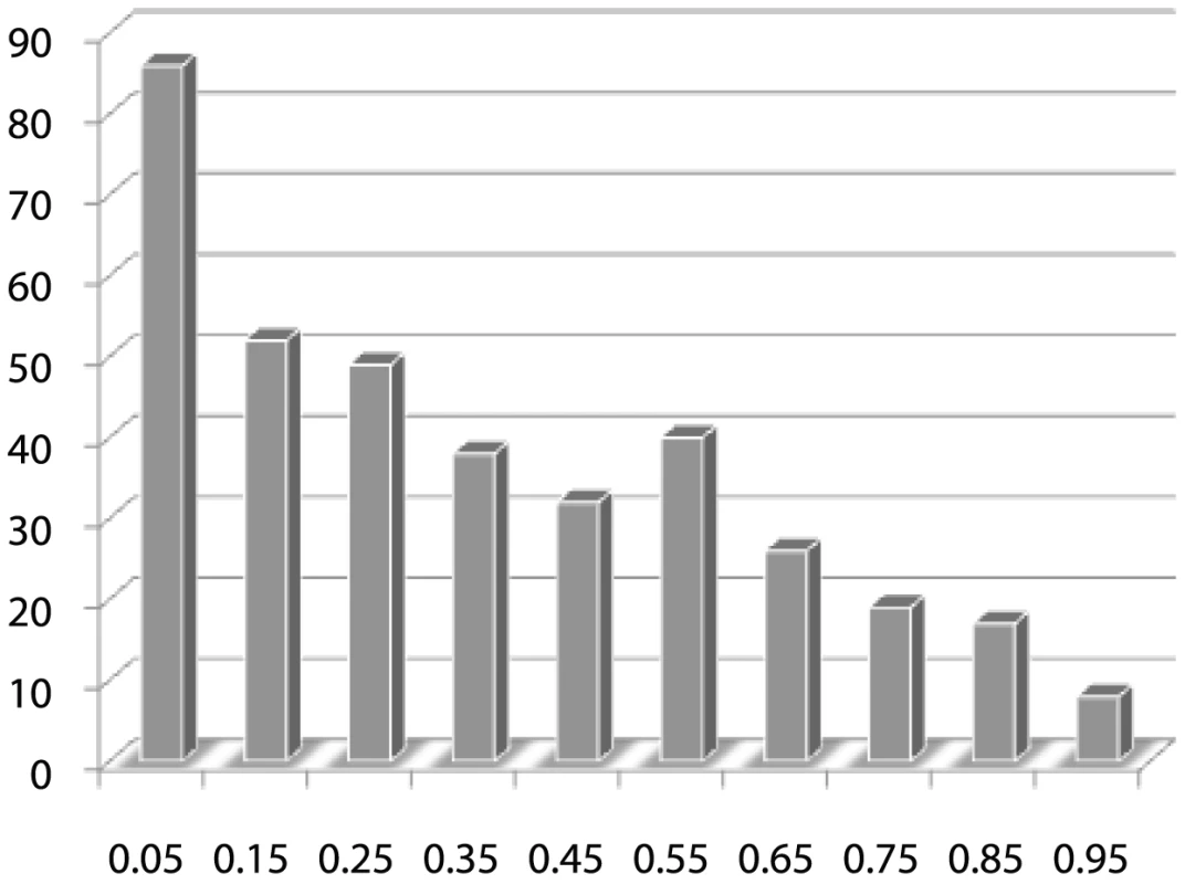
A large value of would suggest that “interesting” genes are more likely to be neighbors. A permutation procedure is used to derive an empirical distribution of under the null hypothesis. The value of an observed is calculated with respect to this empirical distribution. See the Introduction section for more details. In the rest of this article, we first introduce our model and statistical inferential procedures. The performance of our methods is then assessed through both simulation studies and real data applications.
Results
A MRF model of gene pathways
We start by considering a simple model in which a pathway is represented by an undirected graph where is a set of genes (nodes) and are directly connected} denotes the set of all edges. For the th gene in , let denote the set of its neighbors, and denote the number of its neighbors. Let denote the true association status where
The values are referred to as labels of a node hereafter. Let denote the labeling of . Thus is a spatial random vector whose elements may be correlated with each other. Note that each node can be labeled either or , and so there are a total of unique configurations of the pathway. The ultimate goal is to infer the value of based on the pathway topology and the observed association data.
To formalize the idea that neighboring genes tend to have similar association status, we need a probability measure so that nodes connected with each other tend to have the same labels. Here we consider a nearest neighbor Gibbs measure [18] that has the following form:(1)where are the prior parameters or hyperparameters, and are the indicator functions, , and is a normalizing function that is the sum over all possible configurations:(2)
Note that it is prohibitive to evaluate when is large. Here and assign prior weights to edges connecting two non-associated nodes and two associated nodes, respectively. The function will be elaborated in more details in the context of the conditional probability later.
In (1), the second sum is taken over all edges connecting direct neighbors in which both end nodes are labeled −1, and the third sum is taken over all edges in which both end nodes are labeled 1. Positive and will put more weights on configurations in which directly linked nodes have the same labels, which is desirable in our context. The hyperparameter determines the marginal probability of when , i.e., all nodes are treated as singletons that are independent:
The simple form Gibbs measure in (1) has the Markov property that makes it attractive to model a biological pathway, in which directly linked genes interact with each other. It defines a MRF, which by definition is a probability measure that satisfies , where denote all nodes but , and is the set of all direct neighbors of node . Please see Materials and Methods for details.
Posterior distribution
Now we discuss the posterior distribution of association status after combining the evidence from the observed association statistics at the gene level and the structure of the gene pathway. Before we proceed, it is necessary to present the likelihood function of the observed data. We consider the situation where the observed evidence of association is summarized by values, which are assumed to be conditionally independent given the true association status . Under the null hypothesis of no association, each p-value has a uniform (0,1) distribution. In this article, we consider , where and is the CDF (Cumulative Distribution Function) of . Therefore, under the null hypothesis of no association, i.e., , the density of is . However, if there is association between the gene and disease, i.e., , the distribution of is usually unknown. For simplicity, we assume that it is from , where is the location parameter and is the scale parameter that usually depends on the true effect size, allele frequencies, and the sample size. To account for the uncertainty about the parameters, we can put prior distributions on and , and marginalize over them to obtain the predictive density of . Here we consider conjugate priors and , or We denote that are hyperparameters. The prior mean of is and its variance is . The prior mean of is and the prior variance is . This prior is of conjugate form so that the integration over and is analytically tractable. We note that the hyperparameters can be estimated from the observed data via an empirical Bayes method (see Text S2, Figures S1 and S2). Under this prior setting, the marginal density of is
This is equivalent to when 2, and others.
The joint marginal density of is
Thus, the posterior distribution of given the observed data is (3)
Similar to the MRF interpretation of the prior distribution (1), the posterior also has a nice conditional distribution and is actually a MRF, as will be shown in the Materials and Methods section.
When is large, since it is prohibitive to evaluate posterior probabilities on the entire space of configurations, we implement a Markov chain Monte Carlo (MCMC) method to sample from the posterior distribution. Naturally a Gibbs sampler is well suited for a MRF. As will be shown later, due to the MRF property, the posterior has a nice closed-form conditional distribution that can greatly facilitate the MCMC.
Making inference based on the posterior distribution
Most GWAS lead to a set of candidate genes/SNPs that will need to be validated in follow-up studies. Therefore, it is important to include as many truly associated genes as possible among the top ranked genes. Our proposed method allows us to rank order genes as detailed below.
There are several ways of inferring the labels according to the posterior distribution of . The first one is to use maximum a posteriori (MAP) estimate, which is the configuration with the largest posterior probability, a reasonable point estimate for . Let us denote it by . The MAP is the maximizer of the joint posterior distribution:
A Gibbs sampler outlined above can be applied to stochastically search for the solution to the above optimization problem. Multiple restarts with different initial configurations are recommended. An alternative approach is to base the estimate on the posterior conditional probability of given the observed data and all the other nodes . We can estimate by maximizing this conditional probability (MCP): (4)
The advantage of this approach is that the above problem is trivial to solve. As will be explained in equation (8) of the Materials and Methods section, the second term in formula (4) can be evaluated in closed form. Besag [19] proposed an algorithm known as iterated conditional modes (ICM) that iteratively updates . Note that the convergence of ICM is assured because the posterior is proportional to which never decreases at any iteration because the first term is non-decreasing and the second one is a constant. So it is easy to see the ICM will converge to a local maximum in the posterior distribution. Since the ICM runs fast and usually converges in several iterations, multiple restarts with different initial configurations are recommended. Finally the resulting configurations can be compared by evaluating up to a normalizing constant to pick the largest one.
The inference can also be based on the marginal posterior probability. Let . We consider a decision rule in the form , where is an indicator function and is the sought decision threshold. If , the decision is positive (also referred to as discovery) and gene is called to be associated with the disease. Likewise if the decision is negative. To address the problem of multiple comparisons, we consider loss functions associated with making wrong decisions (false discoveries and false negatives), and solve the decision problem by minimizing the expectation of the loss functions under the posterior distribution. Here we consider two loss functions. First, if we are interested in the 0-1 loss function , we may want to minimize the expected loss (5)under the posterior distribution of . The solution is . Note that assigns equal loss to the false positive and false negative errors. This is to minimize the expected frequency of making wrong calls for the association status. Note that the performance of the decision rule is based on the frequentist operating characteristic in the Bayesian framework, which is common in medical decision makings [20]. The second loss function we consider is the false discovery rate (FDR): (6)
Suppose the goal is to control the expected FDR, under the posterior distribution, such that it is no more than , i.e., . If we rank order all genes by their posterior probabilities from the largest to the smallest, and let denote the th order statistics, then the solution is to choose a cut off value where is the largest integer that makes . We should mention that more complicated loss functions can be considered under the framework of our model. See Müller et al. [20] for other examples.
Simulation studies
First we use simulated data to study the performance of the proposed method. The simulation is based on a simple 6-node network shown in Figure 2. Genes G1 through G3 are assumed to be associated with the disease (labeled +1) while G4 through G6 are not associated with the disease (labeled −1). Data are simulated from a disease model as follows. We assume G1, G2 and G3 have independent effects on disease risk and each has a disease related SNP. The genotypes and minor allele frequencies of these three SNPs are denoted by and , respectively, where for A multiplicative genetic model is assumed for the risk of having the disease. More specifically, for an individual with genotype , the risk is , where is the baseline risk of those carrying two normal alleles in all three genes, and is the relative risk, or effect size, of gene , . For each SNP the Hardy-Weinberg equilibrium (HWE) is assumed to hold in the general population so that the genotype probabilities are , , and for , 1, and 2, respectively. In the simulation we use three minor allele frequencies = (0.05, 0.10, 0.15), three disease prevalence values = (0.05, 0.10, 0.15), and six effect sizes = (1.05, 1.10, 1.15, 1.20, 1.25, 1.30). As a result, there are a total of 54 settings of , for each of which we first let and , and then calculate the baseline risk , and finally obtain the conditional distribution of the genotypes given the disease status. Then genotypes of G1, G2 and G3 of 600 cases and 600 controls are simulated according to the conditional genotype distribution. The values of the three causal genes are calculated from a logistic regression of the data. For G4 through G6, the values are simulated from Uniform(0,1). The power of detecting the true association depends on the disease model. In this case, larger values of relative risk, MAF and prevalence corresponds to association tests with higher power.
Fig. 2. A simple 6-node network. 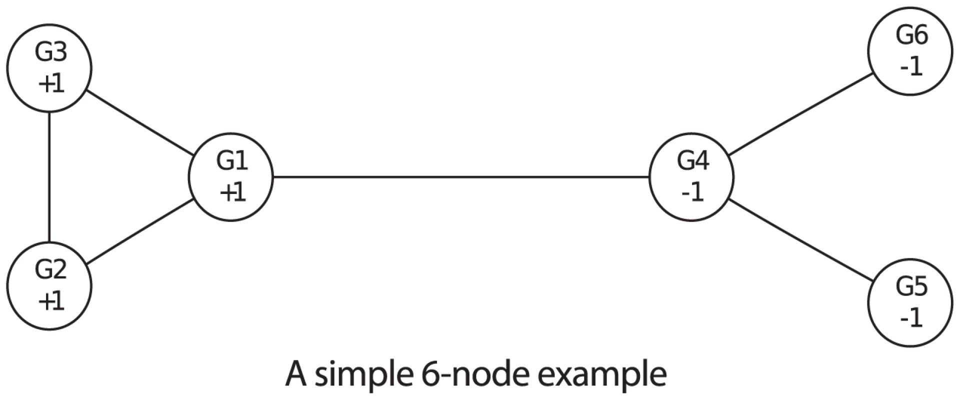
In the simulation we set the hyperparameters = (−1, 0.25, 0.01) where more weights are assigned to edges connecting two associated genes. This corresponds to a prior belief that the probability of association is roughly between 0.35 and 0.50. The hyperparameters are set to (3, 1, 10, 1) where a large value of puts a large prior variance on , which allows a wide range of values for both and . For each simulated data set, the posterior probabilities are enumerated since there are only 64 possible configurations in this simple example. The simulation is repeated 500 times. We compare the proposed method using the posterior mean with the one using the value, and apply cut-off values of 0.7 and 0.05 for posterior probabilities and values, respectively. For each simulated data set, we calculate the false positive rate (FPR), sensitivity (Sens.), and false discovery rate (FDR) by thresholding on values and posterior probabilities. In addition, genes can be rank ordered by the two methods and the area under the Receiver Operating Characteristic curve (AUC) can be calculated. The average values of the three rates plus the AUC over the 500 simulated data sets are shown in Table 1. As can be seen, the proposed method of the posterior probability has higher sensitivity, smaller false discovery rate, and higher AUC than the value thresholding in every setting of the prevalence, MAF and effect size, while the FPR of both methods are controlled at 0.05.
Tab. 1. Average FPR, sensitivities, FDR, and AUC of the 6-node network. 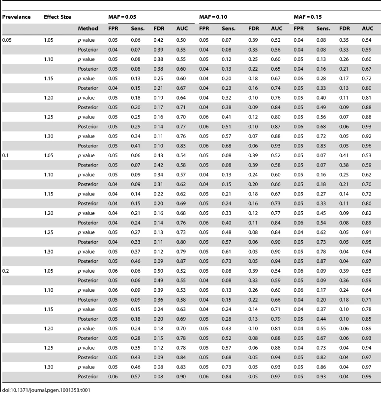
The second simulation study is based on the network shown in Figure 3. This network was adapted from BioCarta “Human Rho cell motility signaling pathway” and we deleted a few genes that are either absent from our Crohn's disease data or not connected to others. We assume three different sets of truly associated genes, plotted in triangles, rectangles and pentagons, each of which contains three, five, and seven nodes, respectively. To simulate different levels in the power of the association tests, for each gene with , the value is computed from a two-sided test where scores are randomly drawn from , and , respectively, corresponding to the power 0.16 (low), 0.32 (median) and 0.51 (high) in the association tests. The values for are generated randomly from Uniform(0, 1) as before.
Fig. 3. A 31-node network adapted from BioCarta “Human Rho cell motility signaling pathway.” 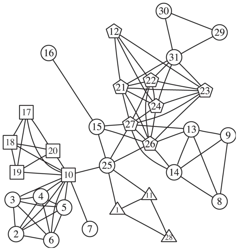
Triangles, rectangles and pentagons denote three different sets of truly associated genes, each of which contains three, five, and seven nodes, respectively. To examine the effects of hyperparameters of the network, we consider eight priors, listed in Table 2, that roughly form four main groups indexed by numbers 1 through 4, and two subgroups indexed by letters and . For each set of hyperparameters a Gibbs sampler is run to draw samples from the corresponding prior distribution, and we can estimate , the prior mean, and and where , the probabilities of edge linking two nodes with identical labels. The averages of the estimated probabilities are listed in the last three columns of Table 2. The average prior means of all nodes are about 0.05, 0.15, 0.25, and 0.4, respectively for the four main groups. Roughly speaking, it means that group 1 is in favor of a small number, and group 4 a large number, while groups 2 and 3 in between, of nodes labeled with +1. Furthermore, values of in subgroup are larger than those in subgroup , meaning that nodes with identical labels are more likely to be next to each other apriori in subgroup than subgroup , as can be seen from the last two columns in Table 2. On the other hand, because the posteriors are found to be insensitive to the hyperparameters when is large, they are set to (3, 1, 10, 1) as in the previous example.
We simulate 200 data sets for each combination of the three power settings (low, median and high) and three truly associated sets (3, 5, and 7 nodes). For each data set, we run eight Gibbs samplers using eight different hyperparameters described above. Each Gibbs sampler is run with 100 restarts and each start contains 100 steps. We compare the average AUC of 200 simulated data sets using value and the posterior mean and plot the results in Figure 4. In general, the AUC of the proposed method is larger than that using values alone. It achieves good AUC if the prior mean is close to the truth, especially when the power is low. For example, in the middle column panels where there are 5 truly associated genes, prior settings 2 and 3, favoring median number of truly associated nodes, outperform prior settings 1 and 4. Similarly, in the right panel where the true model contains 7 genes, prior settings 3 and 4, which are in favor of large models, perform better than the other prior settings. Furthermore, priors in subgroup b are better than subgroup a in general. It is not surprising because the priors in subgroup b encourages nodes labeled with +1 to group together, which agrees with the simulation setting.
Fig. 4. Comparison under different priors. 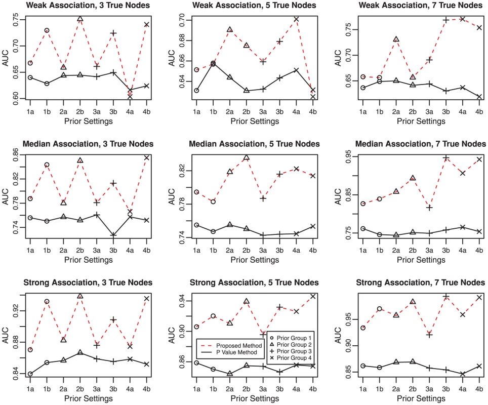
The three rows of panels are for weak (top panel), median (middle panel), and strong (bottom panel) association signals. The three columns of panels are for three sets of truly associated genes corresponding to three (left), five (middle), and seven (right) nodes, respectively. The dotted lines link AUC of the proposed method and the solid lines connect AUC using values. Circles, triangles, plus signs and crosses denote prior parameter groups 1, 2, 3, and 4, respectively. To evaluate the control of the false positive rates and the false discovery rates of the proposed methods in relatively large pathways with only a few associated genes, we conduct a third simulation study based on a simulated network shown in Figure 5 that contains 60 nodes. We consider three truly associated gene sets, namely (2, 11, 19), (2, 11, 19, 41), and (2, 11, 19, 20, 41), and label them as models 1, 2 and 3 in Table 3. Similar to the previous study, we simulate values from scores randomly drawn from , and , corresponding to weak, median and strong associations, respectively. Three prior settings are considered for , namely (−1.5, 0.15, 0.02), (−1.50, 0.10, 0.01) and (−2, 0.2, 0.01), whose average prior probability is approximately 0.2, and average prior probabilities for are roughly 0.13, 0.11, and 0.08, respectively. For the proposed method, we consider three decision rules. The first one (PM1) uses the posterior mean with a cut-off value as in (5), the second one is MCP as in (4), and the third one (PM2) is the method to control the FDR at 0.1 as in (6). Then we compare them with the value method (P value) with a cut-off value set at 0.05 and the correction method (BH) of Benjamini & Hochberg (1995) [21]. For each scenario we simulate 100 data sets, and run a Gibbs sampler with 100 restarts where each start contains 100 iterations. For each simulated data set, we calculate the FPR, sensitivity (Sens.), FDR, and AUC as before. Table 3 lists the average values of the 100 simulation runs. In general PM1 and MCP control the FPR below the 0.05 level and have lower FDR than the value while achieving better or similar power as the value method. In terms of controlling FDR, PM2 controls the FDR around 0.1, and it has smaller FPR or better power than the BH method in most cases when it achieves similar or better FDR.
Fig. 5. A simulated 60-node network. 
Tab. 3. Average FPR, sensitivities, FDR, and AUC of the 60-node simulated network. 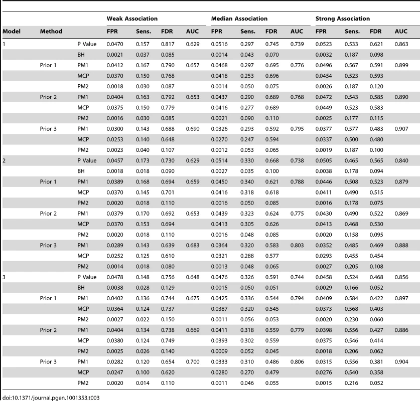
Crohn's disease data
We use one Crohn's disease [15] data set to further evaluate the performance of the proposed method. Details of this data can be found in the Materials and Methods section.
We run our algorithm on 289 pathways that have at least 20 genes with non-missing values. The hyperparameters are chosen such that the average prior mean is roughly between 0.2 and 0.4 based on the simulation findings. To evaluate the performance, we consider 32 target genes that are confirmed to be related to the Crohn's disease [22]. Among these genes, 10 genes can be mapped to 66 pathways. In Figure 6 we plot the AUC values of the rankings by values on the axis and posterior means on the axis for pathways containing three or more target genes. A majority of AUC values are improved if genes are rank ordered by the posterior mean. The average AUC based on values is 0.568 while on posterior means is 0.613. To see what causes the rank changes of genes in the posterior probability, in Figure 7 we show the Human IL-2 Receptor Beta Chain in T cell Activation pathway from BioCarta. Genes in this pathway are densely connected. To aid visualization, we randomly remove some edges. Significant genes whose values are below 0.05 are colored in cyan, genes with improved ranks are colored in light blue and others are colored in pink. It can be clearly seen that genes colored in light blue have more connections with the significant genes, and are more heavily linked among themselves, compared to other genes in the pathway. Genes that have many interactions with each other may play important roles in the biological processes in the pathway. When they are connected to many significant genes, it might be reasonable that they are more likely to associate with the disease than other genes.
Fig. 6. AUC comparison of rankings by values and posterior means for Crohn's disease data. 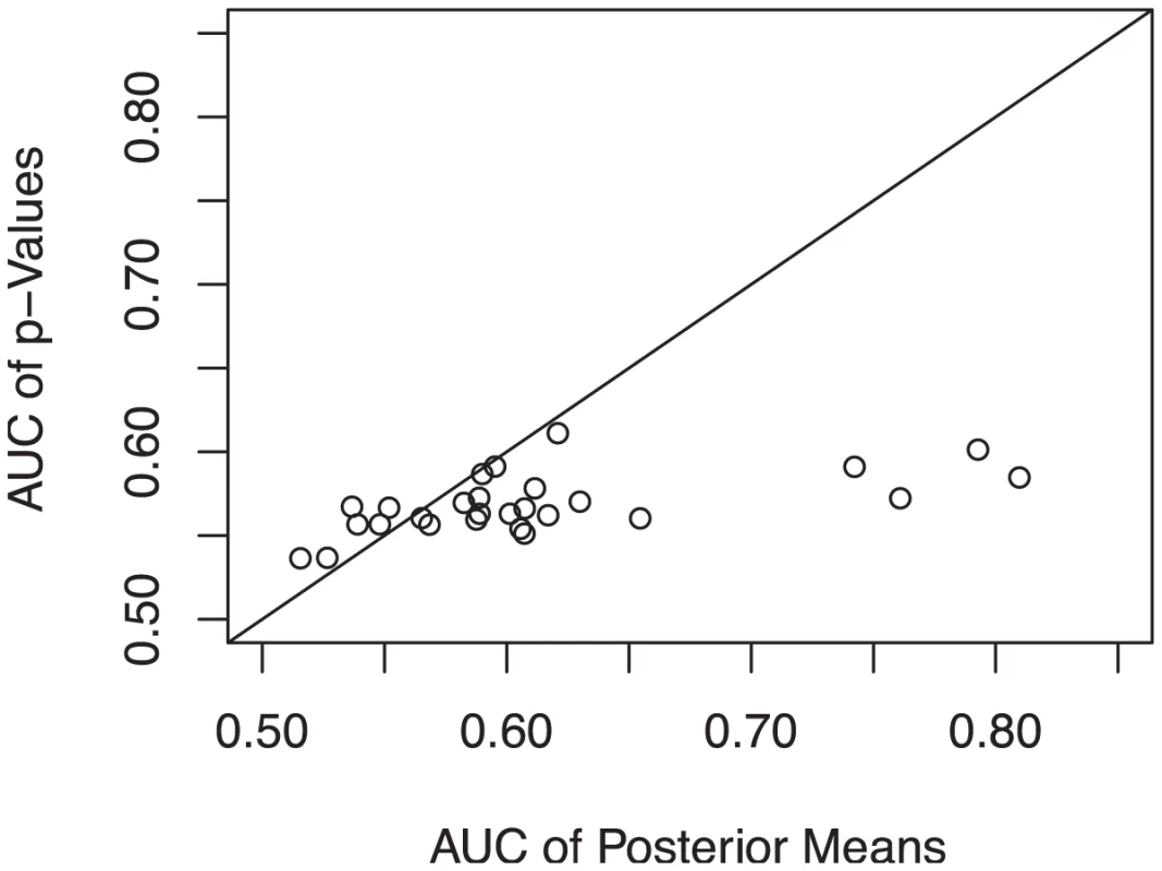
AUC values of the rankings by values are on the axis and that of the posterior means are on the axis for pathways containing three or more target genes. Fig. 7. IL-2 receptor Beta chain in T cell activation pathway. 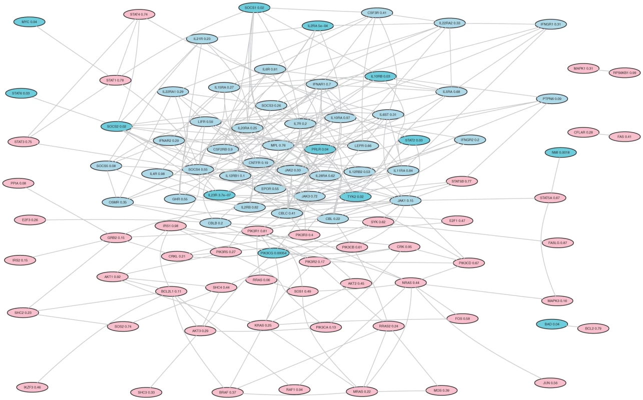
Significant genes whose values are below 0.05 are colored in cyan, genes with improved ranks are colored in light blue and others are colored in pink. Discussion
In this article we introduced a Bayesian method to incorporate prior knowledge of biological pathways into GWAS. This approach uses a MRF as a prior distribution to model the interactions among genes that participate in the same pathway. We showed that the posterior distribution is also a MRF and can be sampled via a Gibbs sampler. Inferences based on the posterior distribution allow us to combine data from the association study with prior information of biological pathways. In particular, this framework considers the topology of all genes in a pathway, which has not been fully utilized in many of the existing methods. The simulation studies and real data example suggest that the proposed method has higher power to identify genes associated with disease.
One limitation of the MRF model is that the Gibbs sampler tends to move around local maxima for a long time and thus can be slow in convergence to the posterior distribution. We recommend to run the Markov chain Monte Carlo with multiple random restarts, and examine the sampling distribution of network statistics, like the number of genes labeled with +1 and the proportion of edges linking genes with identical labels. In our studies, we found that a Markov chain initially moves very rapidly from its starting state, usually within the first 10 to 20 steps, before it reaches some steady states and stabilizes for a long period thereafter. We suggest running 100 Gibbs steps for each random starting state, and conducting the simulation with 100 restarts. The computing time of this scheme typically takes a few minutes on a PC for a pathway of about 30 genes. We should also mention that the characteristics of the MRF defined in (1) depend on both the hyperparameters and the structure of the network under consideration. Consequently there does not exist a set of hyperparameters that can be suitable for all pathways. To assist the specification of hyperparameters, we provide an algorithm of estimating hyperparameters based on a conditional empirical Bayes approach in Text S2. It is recommended that these values would be used in initial attempts and it would be better to test several other variants of hyperparameters, possibly through fine-tuning the initial values. It is helpful to draw samples from the prior distribution to assess the effects o f different prior settings. One limitation of pathway-based analysis is that not all the genes can be associated with pathways. It is likely with knowledge accumulation, more genes will be mapped to pathways. An R package is under construction and will be made publically available soon.
Materials and Methods
The MRF property of the prior distribution on pathways
The nearest neighbor Gibbs measure on gene pathways in formula (1) defines a MRF and its conditional distribution has a logistic regression form as shown below.
Proposition 1
The Gibbs measure in (1) is Markovian and thus defines a MRF
Moreover, the conditional distribution has a logistic form:(7)
where . Equivalently, (7) can be rewritten as a system of linear equations:(8)where
Proof. See Text S1.
This result shows the Markov property that the conditional distribution of , given all other node labels in the network, is equal to the conditional distribution of given all its neighbors. It follows immediately from (8) that if and are not neighbors, then they are conditionally independent.
Now we give an interpretation of . From (8), it is clear that the conditional distribution of depends on the weighted sum of labels of its neighbors, with weight if and if . Here is the sum of weights on both ends of a linking edge. We set to be the square root of of which is the degree of gene . As a result, a gene that interacts with many other genes in the pathway has a large weight because it may play a central role in a biological process and thus it is likely to have a large influence.
The Markovian property of (1) can be derived directly from a more general result [18], which states that a nearest neighbor Gibbs measure is equivalent to a MRF. Our proof that is specific to (1) and is needed to derive the logistic model in (7). We note that under the setting of rectangular lattice systems, Besag [23], [24] presented a general logistic model called the auto-logistic model.
The MRF property of the posterior distribution
To see that the posterior distribution is also a MRF, note that for node ,
Thus, the conditional posterior distribution of given all other nodes only depends on its neighbors, which means the posterior distribution is also a MRF. The conditional posterior log odds of is(9)
where is the marginal likelihood ratio. Therefore, (9) is the product of the marginal likelihood ratio, reflecting the evidence from the data for association with the disease, and the conditional prior odds, reflecting the effect from interactions among neighboring genes from the biological pathway.
To make it clear, we can rewrite (9) in the form of a system of auto-logistic regression equations:(10)where
There are a few observations. First, it is easy to see that the posterior conditional logit form in (9) is the same as the prior conditional logit in (8) except its intercept is . Thus, the observed log likelihood ratio provides a fixed additive effect to the prior logit. Second, the coefficient matrix is symmetric, i.e., . If gene and are not neighbors, then and they are conditionally independent. On the other hand, if they are neighbors, then the impact between each other is equal. Third, genes and are in general correlated in their joint posterior distribution, even if they are not neighbors and are conditionally independent. Moreover, the more common neighbors they share with each other, the stronger the correlation between the two.
The MCMC algorithm
To sample from the posterior distribution, here we implement a Gibbs sampler that is well suited for a MRF. The algorithm is described as follows. First we set an initial value for , say . Then in step , we update the labels sequentially for according to (10): to obtain from . In each cycle we may want to randomize the order in which the nodes are updated.
Crohn's disease data
The Crohn's disease [15] data set is used to evaluate the performance of the proposed method in the Results section. Crohn's disease is a type of inflammatory bowel disease characterized by chronic inflammation of discontinuous segments of the intestine. The disease is found to be related to the interaction of several factors including genetic susceptibility, the intestinal microbial flora of the patient, the patient's immune response to these microbiota, and environmental triggers [25]. It has been well established that Crohn's disease has a strong genetic component [26].
The cohort used in the analysis includes 401 cases and 433 controls. SNPs with a call rate greater than 0.9, minor allele frequency greater than 0.01, and HWE value greater than 0.001 are kept, while subjects with a call rate less than 0.95 are removed from the analysis. Finally 397 cases and 431 controls remain in the analysis. SNPs are considered being mapped to a gene if their physical locations are within 10 kb from the start or end point of the gene as given by Refseq annotation at the NCBI website. Gene level values are obtained by regressing disease status on PCA components that account for at least 85% of the variation [27]–[29]. The pathways and genes in each pathway as well as the gene-level p values can be found at http://bioinformatics.med.yale.edu/group/software.html.
Supporting Information
Zdroje
1. WangK
LiM
BucanM
2007 Pathway-based approaches for analysis of genomewide association studies. Am J Hum Genet 81 1278 1283
2. PengG
LuoL
SiuH
ZhuY
HuP
2010 Gene and pathway-based second-wave analysis of genome-wide association studies. Eur J Hum Genet 18 111 117
3. BallardDH
ChoJ
ZhaoH
2010 Comparisons of multi-marker association methods to detect association between a candidate region and disease. Genet Epidemiol 34 201 212
4. ChunH
BallardD
ChoJ
ZhaoH
2011 Identification of association between disease and multiple markers within a candidate region via sparse partial least squares regression. Submitted
5. FrankeL
van BakelH
FokkensL
de JongED
Egmont-PetersenM
2006 Reconstruction of a functional human gene network, with an application for prioritizing positional candidate genes. Am J Hum Genet 78 1011 1025
6. AertsS
LambrechtsD
MaityS
LooPV
CoessensB
2006 Gene prioritization through genomic data fusion. Nat Biotechnol 24 537 544
7. MaX
LeeH
WangL
SunF
2007 CGI: a new approach for prioritizing genes by combining gene expression and protein-protein interaction data. Bioinformatics 23 215 221
8. HutzJE
KrajaAT
McLeodHL
ProvinceMA
2008 Candid: a flexible method for prioritizing candidate genes for complex human traits. Genet Epidemiol 32 779 790
9. KöhlerS
BauerS
HornD
RobinsonPN
2008 Walking the interactome for prioritization of candidate disease genes. Am J Hum Genet 82 949 958
10. WuX
JiangR
ZhangMQ
LiS
2008 Network-based global inference of human disease genes. Mol Syst Biol 4 189
11. SacconeSF
SacconeNL
SwanGE
MaddenPAF
GoateAM
2008 Systematic biological prioritization after a genome-wide association study: an application to nicotine dependence. Bioinformatics 24 1805 1811
12. WeiP
PanW
2008 Incorporating gene networks into statistical tests for genomic data via a spatially correlated mixture model. Bioinformatics 24 404 411
13. WeiZ
LiH
2007 A Markov random field model for network-based analysis of genomic data. Bioinformatics 23 1537 1544
14. LiH
WeiZ
MarisJM
2010 A hidden markov random field model for genome-wide association studies. Biostatistics 11 139 150
15. DuerrRH
TaylorKD
BrantSR
RiouxJD
SilverbergMS
2006 A genome-wide association study identifies IL23R as an inflammatory bowel disease genes. Science 314 1461 1463
16. SalomonisN
HanspersK
ZambonAC
VranizanK
LawlorSC
2007 Genmapp 2: new features and resources for pathway analysis. BMC Bioinformatics 8 217
17. KanehisaM
GotoS
2000 Kegg: kyoto encyclopedia of genes and genomes. Nucleic Acids Res 28 27 30
18. KindermannR
SnellJL
1980 Markov random fields and their applications. American Mathematical Society ISBN: 0-8218-3381-2
19. BesagJ
1986 On the statistical analysis of dirty pictures. Journal of the Royal Statistical Society Series B (Methodological) 48 259 302
20. MüllerP
ParmigianiG
RobertC
RousseauJ
2004 Optimal sample size for multiple testing: the case of gene expression microarrays. Journal of the American Statistical Association 99 990 1001
21. BenjaminiY
HochbergY
1995 Controlling the false discovery rate: A practical and powerful approach to multiple testing. Journal of the Royal Statistical Society Series B (Methodological) 57 289 300
22. BarrettJC
HansoulS
NicolaeDL
ChoJH
DuerrRH
2008 Genome-wide association defines more than 30 distinct susceptibility loci for Crohn's disease. Nat Genet 40 955 962
23. BesagJ
1972 Nearest-neighbour systems and the auto-logistic model for binary data. Journal of the Royal Statistical Society Series B (Methodological) 34 75 83
24. BesagJ
1974 Spatial interaction and the statistical analysis of lattice systems. Journal of the Royal Statistical Society Series B (Methodological) 36 192 236
25. SartorRB
2006 Mechanisms of disease: pathogenesis of Crohn's disease and ulcerative colitis. Nat Clin Pract Gastroenterol Hepatol 3 390 407
26. PeetersM
NevensH
BaertF
HieleM
de MeyerAM
1996 Familial aggregation in Crohn's disease: increased age-adjusted risk and concordance in clinical characteristics. Gastroenterology 111 597 603
27. GaudermanWJ
MurcrayC
GillilandF
ContiDV
2007 Testing association between disease and multiple SNPs in a candidate gene. Genet Epidemiol 31 383 395
28. WangK
AbbottD
2008 A principal components regression approach to multilocus genetic association studies. Genet Epidemiol 32 108 118
29. BallardDH
2009 Integration of Genomic Data to Identify Genes and Pathways Associated with Disease. Ph.D. thesis, Yale University
Štítky
Genetika Reprodukční medicína
Článek Survival Motor Neuron Protein Regulates Stem Cell Division, Proliferation, and Differentiation inČlánek Epigenetic Regulation of Cell Type–Specific Expression Patterns in the Human Mammary Epithelium
Článek vyšel v časopisePLOS Genetics
Nejčtenější tento týden
2011 Číslo 4- Akutní intermitentní porfyrie
- Farmakogenetické testování pomáhá předcházet nežádoucím efektům léčiv
- Růst a vývoj dětí narozených pomocí IVF
- Pilotní studie: stres a úzkost v průběhu IVF cyklu
- Intrauterinní inseminace a její úspěšnost
-
Všechny články tohoto čísla
- Is Co-Expressed with Closely Adjacent Uncharacterised Genes Spanning a Breast Cancer Susceptibility Locus at 6q25.1
- The Liberation of Embryonic Stem Cells
- Genome-Wide Meta-Analysis Identifies Regions on 7p21 () and 15q24 () As Determinants of Habitual Caffeine Consumption
- A Sustained Dietary Change Increases Epigenetic Variation in Isogenic Mice
- The Exocyst Protein Sec10 Interacts with Polycystin-2 and Knockdown Causes PKD-Phenotypes
- Incorporating Biological Pathways via a Markov Random Field Model in Genome-Wide Association Studies
- Survival Motor Neuron Protein Regulates Stem Cell Division, Proliferation, and Differentiation in
- Identification and Functional Validation of the Novel Antimalarial Resistance Locus in
- Does Positive Selection Drive Transcription Factor Binding Site Turnover? A Test with Drosophila Cis-Regulatory Modules
- Protein Phosphatase 2A Controls Ethylene Biosynthesis by Differentially Regulating the Turnover of ACC Synthase Isoforms
- Ribosomal DNA Deletions Modulate Genome-Wide Gene Expression: “–Sensitive” Genes and Natural Variation
- Reciprocal Sign Epistasis between Frequently Experimentally Evolved Adaptive Mutations Causes a Rugged Fitness Landscape
- Variable Pathogenicity Determines Individual Lifespan in
- Evolution of Vertebrate Transient Receptor Potential Vanilloid 3 Channels: Opposite Temperature Sensitivity between Mammals and Western Clawed Frogs
- Towards Establishment of a Rice Stress Response Interactome
- Mouse Genome-Wide Association and Systems Genetics Identify As a Regulator of Bone Mineral Density and Osteoclastogenesis
- Quantitative Fitness Analysis Shows That NMD Proteins and Many Other Protein Complexes Suppress or Enhance Distinct Telomere Cap Defects
- Highly Precise and Developmentally Programmed Genome Assembly in Requires Ligase IV–Dependent End Joining
- PDP-1 Links the TGF-β and IIS Pathways to Regulate Longevity, Development, and Metabolism
- Genome-Wide Association Study Using Extreme Truncate Selection Identifies Novel Genes Affecting Bone Mineral Density and Fracture Risk
- Eight Common Genetic Variants Associated with Serum DHEAS Levels Suggest a Key Role in Ageing Mechanisms
- 14-3-3 Proteins Regulate Exonuclease 1–Dependent Processing of Stalled Replication Forks
- HDA6 Regulates Locus-Directed Heterochromatin Silencing in Cooperation with MET1
- Epigenetic Regulation of Cell Type–Specific Expression Patterns in the Human Mammary Epithelium
- Enhanced Statistical Tests for GWAS in Admixed Populations: Assessment using African Americans from CARe and a Breast Cancer Consortium
- Beyond Missing Heritability: Prediction of Complex Traits
- An Evolutionary Genomic Approach to Identify Genes Involved in Human Birth Timing
- Long-Lost Relative Claims Orphan Gene: in a Wasp
- PTG Depletion Removes Lafora Bodies and Rescues the Fatal Epilepsy of Lafora Disease
- Chromatin Organization in Sperm May Be the Major Functional Consequence of Base Composition Variation in the Human Genome
- GWAS of Follicular Lymphoma Reveals Allelic Heterogeneity at 6p21.32 and Suggests Shared Genetic Susceptibility with Diffuse Large B-cell Lymphoma
- Loss-of-Function Mutations in Cause Metachondromatosis, but Not Ollier Disease or Maffucci Syndrome
- DNA Damage, Somatic Aneuploidy, and Malignant Sarcoma Susceptibility in Muscular Dystrophies
- The Phylogenetic Origin of Coincided with the Origin of Maternally Provisioned Germ Plasm and Pole Cells at the Base of the Holometabola
- Genome Analysis Reveals Interplay between 5′UTR Introns and Nuclear mRNA Export for Secretory and Mitochondrial Genes
- Genome-Wide Association Analysis of Soluble ICAM-1 Concentration Reveals Novel Associations at the , , , and Loci
- The Complete Spectrum of Yeast Chromosome Instability Genes Identifies Candidate CIN Cancer Genes and Functional Roles for ASTRA Complex Components
- Dynamic Regulation of H3K27 Trimethylation during Differentiation
- Phosphorylation-Dependent Differential Regulation of Plant Growth, Cell Death, and Innate Immunity by the Regulatory Receptor-Like Kinase BAK1
- PLOS Genetics
- Archiv čísel
- Aktuální číslo
- Informace o časopisu
Nejčtenější v tomto čísle- PTG Depletion Removes Lafora Bodies and Rescues the Fatal Epilepsy of Lafora Disease
- Evolution of Vertebrate Transient Receptor Potential Vanilloid 3 Channels: Opposite Temperature Sensitivity between Mammals and Western Clawed Frogs
- Survival Motor Neuron Protein Regulates Stem Cell Division, Proliferation, and Differentiation in
- An Evolutionary Genomic Approach to Identify Genes Involved in Human Birth Timing
Kurzy
Zvyšte si kvalifikaci online z pohodlí domova
Autoři: prof. MUDr. Vladimír Palička, CSc., Dr.h.c., doc. MUDr. Václav Vyskočil, Ph.D., MUDr. Petr Kasalický, CSc., MUDr. Jan Rosa, Ing. Pavel Havlík, Ing. Jan Adam, Hana Hejnová, DiS., Jana Křenková
Autoři: MUDr. Irena Krčmová, CSc.
Autoři: MDDr. Eleonóra Ivančová, PhD., MHA
Autoři: prof. MUDr. Eva Kubala Havrdová, DrSc.
Všechny kurzyPřihlášení#ADS_BOTTOM_SCRIPTS#Zapomenuté hesloZadejte e-mailovou adresu, se kterou jste vytvářel(a) účet, budou Vám na ni zaslány informace k nastavení nového hesla.
- Vzdělávání


