-
Články
- Vzdělávání
- Časopisy
Top články
Nové číslo
- Témata
- Kongresy
- Videa
- Podcasty
Nové podcasty
Reklama- Kariéra
Doporučené pozice
Reklama- Praxe
Dimensionality reduction methods for biomedical data
Authors: Jan Kalina 1; Anna Schlenker 2,3
Authors place of work: Institute of Computer Science CAS, Prague, Czech Republic 1; First Faculty of Medicine, Charles University, Prague, Czech Republic 2; Faculty of Biomedical Engineering, Czech Technical University in Prague, Kladno, Czech Republic 3
Published in the journal: Lékař a technika - Clinician and Technology No. 1, 2018, 48, 29-35
Category: Recenze
Summary
The aim of this paper is to present basic principles of common multivariate statistical approaches to dimensionality reduction and to discuss three particular approaches, namely feature extraction, (prior) variable selection, and sparse variable selection. Their important examples are also presented in the paper, which includes the principal component analysis, minimum redundancy maximum relevance variable selection, and nearest shrunken centroid classifier with an intrinsic variable selection. Each of the three methods is illustrated on a real dataset with a biomedical motivation, including a biometric identification based on keystroke dynamics or a study of metabolomic profiles. Advantages and benefits of performing dimensionality reduction of multivariate data are discussed.
Keywords:
biomedical data, dimensionality, biostatistics, multivariate analysis, sparsityIntroduction
The aim of this paper is to present basic principles of common dimensionality reduction methods, to charac-terize main approaches to dimensionality reduction and to illustrate selected methods and their benefits on real data with a biomedical motivation. We choose here three particular approaches and describe them in detail. These are important as well as reliable examples of three main types of dimensionality reductions.
- Principal component analysis (PCA), which represents the most common feature extraction method in biomedical applications;
- Minimum redundancy maximum relevance (MRMR) approach, which is a variable selection method; and
- Nearest shrunken centroid (NSC), which is an exam-ple of a sparse classification method (classifier) with an intrinsic variable selection.
While the scope of this paper must stay limited, numerous other methods can be found in specialized literature [1–3].
Reducing the dimensionality of biomedical data be-comes extremely needed with the increasing availability of Big Data in biomedicine and healthcare [4]. A pre-processing and cleaning of multivariate data together with a subsequent dimensionality reduction and explor-atory data analysis represent crucial preliminary steps of their analysis [2, 5]. Thus, dimensionality reduction does not represent the very aim of the data analysis, but rather a preparatory (auxiliary) tool with the aim to find the most important variables or some latent factors or components behind the data (possibly with a clear interpretation). Their subsequent analysis, often guided by the main task from the perspective of the biomedical problem under consideration, may have different one of the following main aims:
- Classification (the task to assign a new observation to one of given groups, based on a training dataset with a known group labeling);
- Regression (explaining and predicting one or more variables by means of other variables);
- Clustering (finding natural groups of data, without a prior knowledge of these groups);
- Clinical decision support within decision support systems [6, 7].
Dimensionality Reduction
Some form of dimensionality (or complexity) reduction is commonly used as a preliminary step of analyzing complex data. The aim of this section is to discuss dimensionality reduction from a general per-spective, to overview our experience from various practical biomedical analyses and to characterize its important types. Examples of particular methods will be then described in the following sections, where the methods were selected as flagships (prominent and at the same time reliable even in the simplest version) of the main types of dimensionality reduction.
In the whole paper, we assume that the total number n of p-dimensional observations (random vectors, measurements) is observed, where the j-th observation (sample) is denoted as Xj1,…,Xjp for j=1,…,n. The data may be continuous and/or categorical and the observed variables may correspond to symptoms and signs or laboratory measurements. If p is large, and especially if p exceeds n largely (i.e. n≪p), we speak of high-dimensional data.
If the data are high-dimensional data, standard statistical methods suffer from the so-called curse of dimensionality and dimensionality reduction becomes a necessity. The serious challenges include not only the high dimensionality itself, but also the presence of outliers, dependence among variables, or the need to combine continuous and categorical variables [3]. Only recently, biomedical researchers seem to be becoming aware of dimensionality reduction methods tailor-made for high-dimensional data [8–11]. These have been proposed not only in journals focused on biostatistics or multivariate statistics, but also in those devoted to information theory, computer science, or bioinformatics.
Examples of real-world biomedical applications, where dimensionality reduction brings benefits, include:
- Analysis of spontaneous and induced neuronal oscillations in brains in schizophrenia patients and healthy controls, and particularly performing a pre-processing to clearly separate signal and noise [12];
- Finding predictors of age of a tissue based on DNA methylation products [13];
- Human identification based on infrared images of the iris, particularly searching for features with the largest discrimination ability [14].
In general, dimensionality reduction may bring various benefits:
- Simplification of a subsequent analysis, i.e. allowing to compute standard statistical methods, which would be either computationally infeasible or at least numerically unstable under the presence of redundant variables [15];
- Improving the interpretation of consequent analysis;
- Decorrelation, i.e. reducing or removing correlations (associations) among variables, which improves the stability of a subsequent analysis;
- Describing differences among given groups;
- Revealing the dimensionality of the separation among given groups, e.g. by expressing the contribution of individual variables to the separation among given groups;
- Dividing variables to clusters [16];
- A possible improvement of the performance of a subsequently performed classification (which is possible but definitely not typical).
We distinguish between supervised and unsupervised dimensionality reduction methods. Supervised ones are tailormade for data coming from two or more groups, while the information about the group membership is taken into account. We denote by (?1,…, ??)? the grouping variable corresponding to the true group membership of the observed data, where ?? = 1 if the
i-th observation comes from the first group and ?? = 0 otherwise. Unsupervised methods consider data only in one group. If the data are in groups but the group labeling is not known even for the training dataset, unsupervised methods must be used. It is suboptimal to use an unsupervised approach for data coming from several known groups.We also distinguish between prior variable selection (also denoted plainly as variable selection or feature selection), which selects a smaller set of important variables and ignores all remaining ones, and feature extraction, which replaces the data by combinations of variables. A specific category of variable selection methods are sparse approaches, which contain an intrinsic variable selection and the subsequent analysis ignores some of the variables; also future measurements in the same situation can be performed on a smaller set of variables, which may reduce the (e.g. financial) demands of the experiments.
It is not possible to give a general answer to the question which approach is the best for a given dataset. Of course, each method has its own set of assumptions. Feature extraction (unlike variable selection) ensures decorrelation and consequently a better stability of the results. Correlations of variables do not have a harmful influence on predictions and if the user is interpreted in predictions, feature extraction is usually suitable even without a clear interpretation of the result.
On the other hand, variable selection may be the preferable choice if a clear interpretation is desirable. It induces sparsity, i.e. the user does not have to measure all variables. It allows to give comprehensible answers to various questions, e.g. how to explain values of individual parameters or which variables are the most important ones (for explaining the odds ratio that a disease will develop etc.).
Principal Component Analysis
Principal component analysis (PCA) represents the most commonly used feature extraction method [1]. After we describe the method, PCA will be illustrated on a small dataset.
Method
We denote here the i-th variable as Xi=(
X1i,…,Xni)T for i=1,…,p. The method considers the empirical covariance matrix S of the data defined as Here, ? denotes the p-dimensional arithmetic mean of the observations. The whole PCA is based on algebra transforms of the (symmetric) matrix S. Particularly, the so-called eigenvalues λ1,…,λp of S, which are all non-negative, and their corresponding eigenvectors denoted as q1,…,qs will be used. The idea is to explain each observation as the mean (across all observations) plus the individual effect evaluated as a linear combination of the principal components, where the most variables ones (most remarkable) are the first ones.
The aim of PCA is to replace the p-dimensional observations by a small set of principal components. Let us say that the transformed data will be s-dimensional, where s<min(n,p). This means replacing the original p variables by transformed variables Z1,…,Zs, where the i-th variable contains values denoted as Zi=(
Z1i,…,Zni)T for i=1,…,p. The original measure-ments are replaced by new transformed measurements in the form of linear combinations of the observed values. The j-th one is denoted here as (Zj1,…,Zjs)T and Zji is obtained as The new variables are mutually uncorrelated, i.e.
It holds that
i.e. the important components in terms of explaining the variability of the transformed data are the first ones, and moreover it holds that var Zi=λi for i=1,…,s. The contribution of the i-th principal component (corresponding to the i-th largest eigenvalue) to explaining the total variability in the transformed data can be expressed as λi divided by the total variability evaluated as var X1 +…+var Xp, where i=1,…p.
Reducing the number of transformed variables only to s may bring a remarkable reduction of computational costs, especially if the constant s is much smaller than p. The user may require the variability of the selected principal components to be at least a given percentage (e.g. 80 %) of the total variability of the data. This determines how to choose an appropriate s. Alterna-tively, principal components may be computed from the empirical correlation matrix, which may be recom-mended only in case of big differences in variability of individual variables [1].
The computation of PCA may be performed in a numerically stable way also for high-dimensional data, although software contains also unstable imple-mentations. Therefore, specialized packages suitable for PCA for high-dimensional data are available, e.g. libraries HDMD or FactoMineR of R software [17].
Example 1
We analyze a real data acquired within a multifactor authentication system to electronic health record security [18]. We focus on its particular procedure for person authentication, which exploits keystroke dynamics. Here, we work only with a subset of the data from a larger study so that we illustrate some computations. We consider the data measured only on 2 probands, who were asked to write the word “kladruby” 5-times, each time in the habitual speed. The authentication is a classification task to 2 groups with n=10, where there are p=15 variables including 8 keystroke durations (periods of time of holding a particular key) and 7 keystroke latencies (periods of time between holding two individual consecutive keystrokes) measured in milliseconds.
We use the classification by means of a support vector machine (SVM) classifier [15], which is a machine learning tool theoretically founded with a good performance also for high-dimensional data [19]. A linear SVM is able to classify each observation correctly also in a leave-one-out cross validation (LOOCV) study. Within a LOOCV, which can be described as an attempt for an independent validation, an observation is left out, the classification rule is learned over the remaining data and the classification of the observation being left out is performed. This is repeated over all observations and the overall classification accuracy is evaluated, which is defined as the percentage of correctly identified samples, i.e. ratio of correctly classified observations divided by n. In this terminology, the classification accuracy of the linear SVM is equal to 1.0 in the LOOCV.
However, it is not possible to perform the classification e.g. by means of linear discriminant analysis (LDA), which is a popular comprehensible classifier based on distances of observations from the means of each group [1], because n is smaller than p in this example. Let us perform a more detailed study of the classification ability of individual principal components. This time, the classification will be performed by the LDA rather than by the much more complicated SVM method. Table 1 evaluates the contribution of the 9 principal components to the separation between both groups based on individual components and pairs of components (first together with the second etc.). The separation performance here is evaluated as the classification accuracy of LDA within a LOOCV study.
Tab. 1. A study of principal components of the keystroke dynamics data in Example 1. Classification accuracy of LDA evaluated in a LOOCV study exploiting (1) individual principal components, (2) pairs of two principal components, and (3) the cumulative contribution of components {1,…,r} for each r=1,…,9. 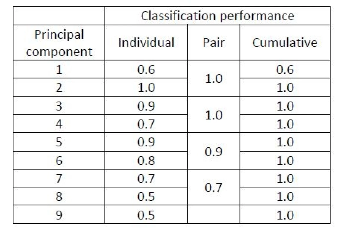
The following principal components have a better ability to separate the two groups. The 3rd and the 4th principal components are shown in Figure 2. Their variability is smaller but their contribution to the classification is higher compared to the very first principal component.
Fig. 1. The 1st and 2nd principal component in Example 1 in group 1 (empty circles) and group 2 (full cirlces). 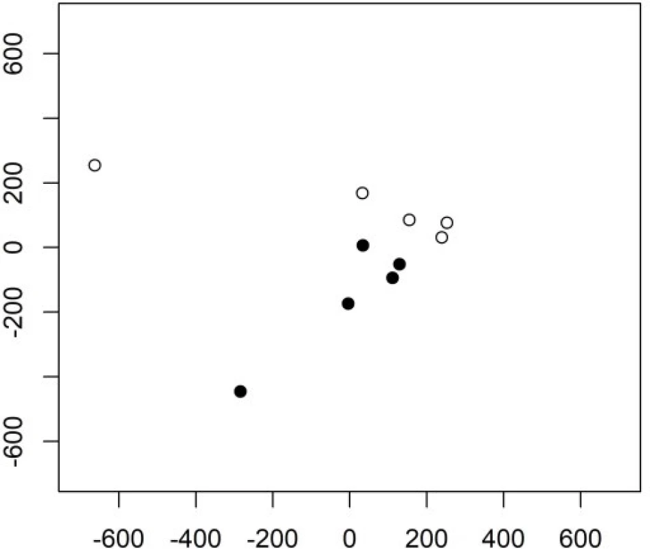
Fig. 2. The 3rd and 4th principal component in Example 1 in group 1 (empty circles) and group 2 (full circles). 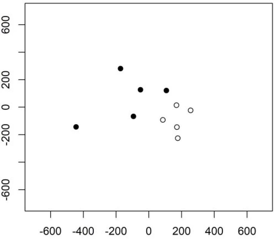
Keystroke latencies in the word “kladruby” turn out to be much more important for the classification task compared to keystroke durations. We will denote the keystroke latency e.g. between releasing key a and pressing key d as ad. The first principal component can be (with some level of simplification) interpretetd as ad+ru-dr-ib, the second as ad+ru-la. Both contain the latencies ad and ru which thus turn out to be crucial for the classification task.
In this example, a small number of components carries the information important for the classification. The very first one principal component does not, but still this enables the PCA to be useful here. Indeed, PCA is often (and successfully) used also for data in groups (although it is designed as an unsupervised method) [9]. In general, however, the interpretation of the principal components, may be more difficult.
MRMR Variable Selection
Method
The minimum redundancy maximum relevance (MRMR) methodology represents a class of supervised variable selection tools [20]. We describe the principles for analyzing p-dimensional data coming from two groups. The advantage of the approach is that it does not incline to selecting strongly correlated variables. The method requires to measure relevance of a set of variables for the classification task, i.e. to evaluate the contribution of a given variable to the classification task. Also it is necessary to use a measure of redundancy of a set of variables. We use here the mutual information as the measure of both relevance and redundancy. This however requires all variables in the given dataset to be categorical. If these are continuous, they must be first transformed to categorical variables. An alternative approach would be to use other measures based on information theory, specific test statistics or p-values, or very simple ad hoc criteria [21].
The index corresponding to the group label will be denoted as an indicator variable Y (as above). The procedure selects gradually one variable after another and these form a set denoted as S. First, we need to evaluate for each variable (say Z) its relevance for the classification task, which will be denoted as Relevance (
Here, α∊(0,1) is a chosen parameter and S∪Z denotes the set of variables included so far in S together with the variable Z. Such variable is selected to the set S, which maximizes (5).
We can say that relevance in (5) is penalized by means of the redundancy. The selection of variables according to (5) is repeated and new variables are added to the set of selected variables until a given stopping rule is fulfilled. The user may either choose a fixed number of relevant variables, or he/she may require that the selected variables contribute to explaining more than a given percentage (e.g. 90 %) of the interclass variability of the observed data.
The value of α can be chosen to maximize the classification accuracy and a leave-k-out cross valida-tion represents a popular choice here (mainly with k=1), which is performed in the following way. For a fixed α, there are k randomly chosen observations left out, the classifier is computed and the observation left out are classified. This is repeated sufficiently many times and the overall classification accuracy is evaluted. The whole procedure is repeated for various α and such its value is selected as the optimal one, which yields the maximal classification accuracy.
Example 2
The performance of the MRMR variable selection is illustrated on a data set from the biometric authentication, which is however different from that of Example 1. Again, the probands were asked to type the word “kladruby” 5-times at the habitual speed. Here however we work with data from 32 probands, so our analysis goes beyond the results of [21]. In the practical application, one of the 32 individuals identifies himself/herself (say as ??) and types the password. It would be possible to consider a classification task to 32 groups. Nevertheless, the task within the practical problem is different. An individual claims to be a given person (say XY) and the system has the aim to verify if this is true. Such authentication (rather than recognition) task is a classification problem to assign the individual to one of the ? = 2 groups performed with p=15 and n=32*5=160.
If all variables are used with a linear SVM, the classification accuracy is equal to 0.93. The following analysis is peformed with the LDA classifier, which is much simpler than the SVM approach. If the dimensionality of the data is reduced, the SVM classifier has a tendency to overfitting, because it is not designed for data with a small n.
If only 4 variables selected by MRMR are used, the classification accuracy of the LDA is 0.93 in a LOOCV study. Keystroke latencies again turn out to be more important than keystroke durations by the MRMR criterion. The most important variables according to the MRMR criterion are ad, ru, dr, and ub. If only the variable ad is used, the classification accuracy of the LDA linear SVM in the LOOCV is 0.57. If ad and ru are used together, it increases to 0.82. The first three of these variables yield 0.90 and all four yield already 0.93. On the whole, MRMR does not improve classification but loses only a little and allows to find the most relevant variables for the classification task.
One may ask about an alternative idea based on selecting only variables with the largest variability. This would be an unsupervised approach. The variables with the largest variability are ub and by, but constructing a classification rule based mainly on them would be misleading. LDA using these two variables gives namely the classification accuracy 0.55 in a LOOCV.
Nearest Shrunken Centroid (NSC)
Method
The method called Shrunken Nearest Centroid (NSC) is a supervised classification method proposed by [22] originally for high-dimensional data in molecular genetics. In contrast to previously describe methods reducing the dimensionality prior to classification tasks, the NSC performs a variable selection intrinsically (as its integral part). Thus, the resulting classification rule depends only on a certain number of variables (i.e. induces sparsity), while the influence of the remaining variables is suppressed, possibly even to zero.
The task is to learn a classification rule to K groups and the classification rule of the NSC is based on distances of a new observation Z from the centroid of each of the groups. The centroid (prototype) denoted as
is minimal. Here, si is the standard deviation of the i-th variable, s0 is a positive constant, and pk is a prior probability of observing from the k-th group. The centroid
Fig. 3. Explanation of the NSC classifier on an artifical dataset with data in two groups. The arithmetic mean (center of gravity, shown as a full circle) of each group is shrunken towards to the overall mean (across groups). 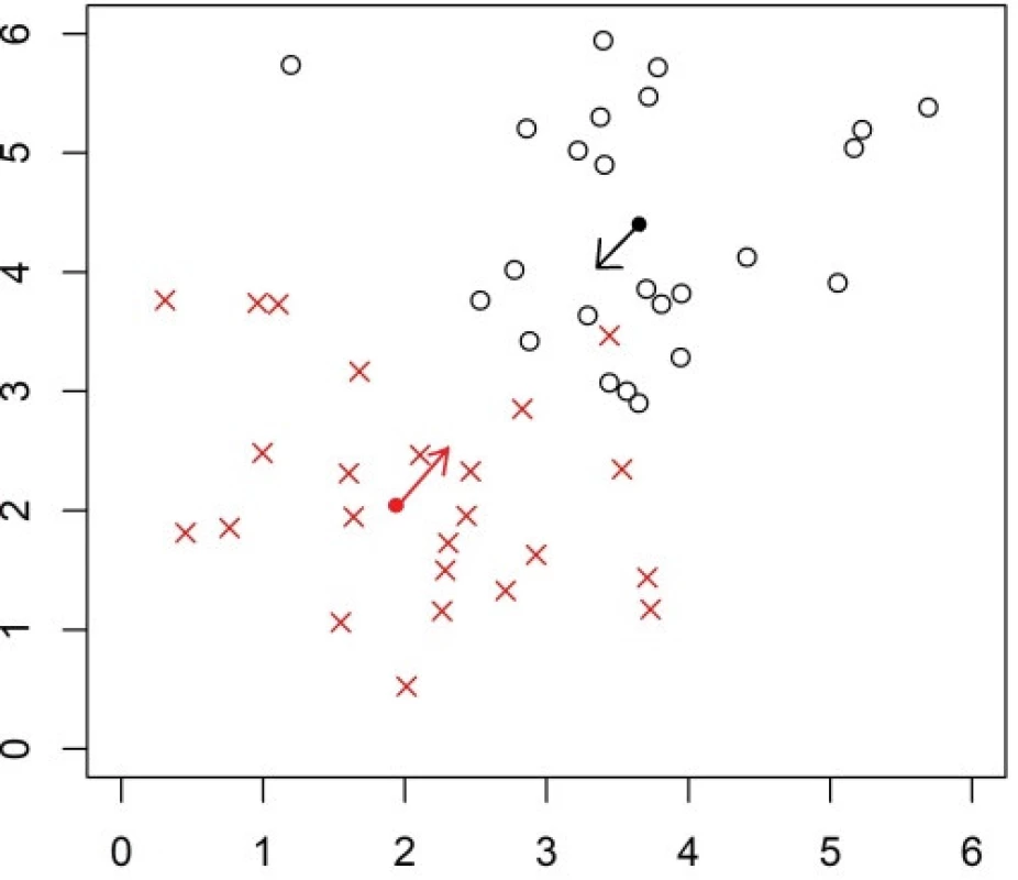
Tab. 2. Results of Example 3. Classification accuracy obtained with the NSC for the metabolomic profiles dataset for various values of λ, i.e. for various numbers of variables relevant for the classification rule. 
The value of Xik depends on a parameter λ called shrinkage intensity, which determines the level of shrinkage of the mean towards the overall mean. The classification rule does not depend on all variables, but some are ignored, and a larger λ leads to ignoring more variables. The NSC arranges all variables according to their contribution to the classification task [22]. A LOOCV can be applied to find a suitable value of λ, which determines the level of shrinkage of the estimator. Such value is selected, which leads to the maximal classification accuracy. If there are several values of the threshold yielding the same accuracy, then the minimal value among them is selected. Numerical experiments of [22] revealed advantages of the NSC over standard methods especially when there are more than two classes.
Example 3
We analyze a popular benchmarking dataset of prostate cancer metabolomic data [23] of p=518 metabolites measured over two groups of patients, who are either those with a benign prostate cancer (16 patients) or with other cancer types (26 patients). The dataset is publicly available in the MPINet library of R package [24].
Conclusions
This paper overviews principles and types of dimensionality reduction approaches, presents three selected methods important for biomedical applications and illustrates their performance on real datasets. The examples are motivated by our attempt to persuade the reader about the potential of reducing the dimensionality of multivariate data. Dimensionality reduction is claimed to be beneficial for various types of data and various analysis tasks.
In the keystroke dynamics examples of this paper, a small set of variables or their components turns out to carry the majority of the information relevant for the classification task. Also for the high-dimensional metabolomic data [23], a set of 21 variables seems sufficient.
In the presented datasets, the data are observed in two groups and the task is to learn a classification rule over a training dataset. The dimensionality reduction itself does not improve the classification results here, but still is very beneficial in these examples. It namely allows to use much more suitable classification methods in terms of comprehensibility only at the price of a small reduction of the classification performance and (at least for some methods) to improve the interpretation of subsequent data analysis.
Numerous available tools for dimensionality reduction, which exceed the scope of this paper, belong to the important classes mentioned here: feature extraction, prior variable selection, or sparse variable selection. Particularly for high-dimensional data, there remains an unflagging interest in proposing new methods, especially exploiting principles of sparsity explained on the example of the NSC in this paper. Other recent research topics include combination of various data types [25] or comparisons of various dimensionality reduction methods, however usually performed in more specific tasks [26] or within only a narrower class of dimensionality reduction tools [27].
Acknowledgements
The work was partially supported by the PROGRESS Q25, Charles University, Prague, and by the project NV15-29835A of the Czech Health Research Council.
RNDr. Jan Kalina, Ph.D.
Institute of Computer Science of the Czech Academy of Sciences
Pod Vodárenskou věží 2, 182 07 Praha 8
Czech Republic
E-mail: kalina@cs.cas.czIng. Anna Schlenker
Institute of Hygiene and Epidemiology
First Faculty of Medicine
Charles University
Studničkova 7, 128 00 Praha 2
&
Faculty of Biomedical Engineering
Czech Technical University in Prague
nám. Sítná 3105, 272 01 Kladno
Czech Republic
E-mail: schlenker.anna@gmail.co
Zdroje
- Rencher, A. C.: Methods of multivariate analysis. Second edn. Wiley, New York, 2002.
- Dziuda, D. M.: Data mining for genomics and proteomics: Analysis of gene and protein expression data. Wiley, New York, 2010.
- Fan, J., Lv, J.: A selective overview of variable selection in high dimensional feature space. Statistica Sinica, 2010, vol. 20, pp. 101–148.
- He, M., Petoukhov, S.: Mathematics of bioinformatics: Theory, methods and applications. Wiley, Hoboken, 2011.
- Luo, J., Wu, M., Gopukumar, D., Zhao, Y.: Big data application in biomedical research and health care: A literature review. Biomedical Informatics Insights, 2016, vol. 8, pp. 1–10.
- Zvárová, J., Veselý, A., Vajda, I.: Data, information and knowledge. In Berka, P., Rauch, J., Zighed, D. (eds.): Data mining and medical knowledge management: Cases and applications standards. IGI Global, Hershey, 2009, pp. 1–36.
- Venot, A., Burgun, A., Quantin, C. (eds.): Medical informatics, e-health. Fundamentals and applications. Springer, Paris, 2014.
- Tan, Y., Shi, L., Tong, W., Hwang, G. T. G., Wang, C.: Multi-class tumor classification by discriminant partial least squares using microarray gene expression data and assessment of classification models. Computational Biology and Chemistry, 2004, vol. 28, pp. 235–244.
- Duintjer Tebbens, J., Schlesinger, P.: Improving implementation of linear discriminant analysis for the high-dimensional/small sample size problem. Computational Statistics and Data Analysis, 2007, vol. 52, pp. 423–437.
- Bartenhagen, C., Klein, H. U., Ruckert, C., Jiang, X., Dugas, M.: Comparative study of unsupervised dimension reduction tech-niques for the visualization of microarray gene expression data. BMC Bioinformatics, 2010, vol. 11, Article 567.
- Matloff, N.: Statistical regression and classification. From linear models to machine learning. CRC Press, Boca Raton, 2017.
- Haufe, S., Dähne, S, Nikulin, V. V.: Dimensionality reduction for the analysis of brain oscillations. NeuroImage, 2014, vol. 101, pp. 583–597.
- Lee, J., Ciccarello, S., Acharjee, M., Das, K.: Dimension reduc-tion of gene expression data. Journal of Statistical Theory and Practice, 2018, online first, in press.
- Tan, C. W., Kumar, A.: Unified framework for automated iris segmentation using distantly acquired face images. IEEE Transactions on Image Processing, 2012, vol. 21, pp. 4068–4079.
- Hastie, T., Tibshirani, R., Wainwright, M.: Statistical learning with sparsity: The lasso and generalizations. CRC Press, Boca Raton, 2015.
- Bushel, P., Wolfinger, R. D., Gibson. G.: Simultaneous clus-tering of gene expression data with clinical chemistry and pathological evaluations reveals phenotypic prototypes. BMC Systems Biology, 2007, vol. 1, Article 15.
- McFerrin, L.: Package HDMD. R package version 1.2 (2013).
- Schlenker, A., Tichý, T.: A new approach to the evaluation of local muscular load while typing on a keyboard. Central European Journal of Public Health 2017, vol. 25, pp. 255–260.
- Vapnik, V. N.: The nature of statistical learning theory. Second edn. Springer, New York, 2000.
- Ding, C., Peng, H.: Minimum redundancy feature selection from microarray gene expression data. Journal of Bioinformatics and Computational Biology, 2005, vol. 3, pp. 185–205.
- Kalina, J., Schlenker, A.: A robust supervised variable selection for noisy high-dimensional data. BioMed Research International, 2015, vol. 2015, Article 320385.
- Tibshirani, R., Hastie, T., Narasimhan, B., Chu, G.: Class predic-tion by nearest shrunken centroids, with applications to DNA microarrays. Statistical Science, 2003, vol. 18, pp. 104–117.
- Sreekumar, A. et al.: Metabolomic profiles delineate potential role for sarcosine in prostate cancer progression. Nature, 2009, vol. 457, pp. 910–914.
- Xu, Y., Li, C., Li, X.: Package MPINet. R package version 1.0 (2015).
- Viswanath, S. E., Tiwari, P., Lee, G., Madabhushi, A., Alz-heimer’s Disease Neuroimaging Initiative: Dimensionality reduction-based fusion approaches for imaging and non-imaging biomedical data: Concepts, worksflow, and use-cases. BMC Medical Imaging, 2017, vol. 17, Article 2.
- Harikumar, R., Kumar, P. S.: Dimensionality reduction tech-niques for processing epileptic encephalographic signals. Biomedical & Pharmacology Journal, 2015, vol. 8, pp. 103–106.
- Xie, H., Li, J., Zhang, Q., Wang, Y.: Comparison among dimensionality reduction techniques based on Random Projection for cancer classification. Computational Biology and Chemistry, 2016, vol. 65, 165–172.
Štítky
Biomedicína
Článek vyšel v časopiseLékař a technika

2018 Číslo 1-
Všechny články tohoto čísla
- Median method for determining cortical brain activity in a near infrared spectroscopy image
- Patient´s respiratory curve synchronization by visual feedback application
- A comparsion of the quality of dental crowns from TI-6AL-4V and cocr alloys made with SLM technology
- Dimensionality reduction methods for biomedical data
- Agcu bimetallic nanoparticles modified by polyvinyl alcohol - the cells viability study in vitro
- Lékař a technika
- Archiv čísel
- Aktuální číslo
- Informace o časopisu
Nejčtenější v tomto čísle- Median method for determining cortical brain activity in a near infrared spectroscopy image
- A comparsion of the quality of dental crowns from TI-6AL-4V and cocr alloys made with SLM technology
- Dimensionality reduction methods for biomedical data
- Patient´s respiratory curve synchronization by visual feedback application
Kurzy
Zvyšte si kvalifikaci online z pohodlí domova
Autoři: prof. MUDr. Vladimír Palička, CSc., Dr.h.c., doc. MUDr. Václav Vyskočil, Ph.D., MUDr. Petr Kasalický, CSc., MUDr. Jan Rosa, Ing. Pavel Havlík, Ing. Jan Adam, Hana Hejnová, DiS., Jana Křenková
Autoři: MUDr. Irena Krčmová, CSc.
Autoři: MDDr. Eleonóra Ivančová, PhD., MHA
Autoři: prof. MUDr. Eva Kubala Havrdová, DrSc.
Všechny kurzyPřihlášení#ADS_BOTTOM_SCRIPTS#Zapomenuté hesloZadejte e-mailovou adresu, se kterou jste vytvářel(a) účet, budou Vám na ni zaslány informace k nastavení nového hesla.
- Vzdělávání


