-
Medical journals
- Career
On mixed statistical moments of texture in ultrasound B-mode images
Authors: Jaromír Šrámek 1,2; Jiřina Škorpíková 2
Authors‘ workplace: Department of Biophysics, Faculty of Medicine, Masaryk University Brno, Czech Republic 1; Pathology, Hospital Jablonec n/N, Jablonec nad Nisou, Czech Republic 2
Published in: Lékař a technika - Clinician and Technology No. 2, 2013, 43, 13-16
Category: Original research
Overview
Texture is one of the most important propeties of ultrasound image. Because subjective evaluation of there is limited by the lack of capability of a natural language to rigorous description of texture, there are used a wide spectrum of texture descriptors. In the viewpoint of mathematics is texture of an object in the digital image generally a discrete stochastic process. Texture of the concrete object is thus the realization of this stochastic process. It shows, in some mathematical simplifications, of course, the possible way to compare of two textures. In this work, we analyzed the usefulness of mixed statistical moments of textured pattern in ultrasound image. The main result is that mixed moments may be useful to texture analysis of ultrasound images. A little bit surprising is relatively high sensitivity of mixed moments on anisotropy of ultrasound images.
Keywords:
medical ultrasound, texture analysis, statistical momentsIntroduction
The medical ultrasound is a widely used medical device because of its low cost, low exposure of patients, and, last but not least, relatively simple use [1]. The typical ultrasound image is formed by the so called speckles [1]. The speckles give the image characteristic “dotted” pattern [1] which is a seductive goal for texture analysis. Accordingly, the first works deal with texture analysis of ultrasound images have been written in the late 1970s [2].
Texture
Texture is a property of a surface which is more complex than color properties. [3] Texture contains not only the information about color and lightness of a surface but also the information about structure of the surface. There is not any generally accepted and widely used definition of texture, there is used for each task the relatively specific conception [4]. For example, the conception of texture as a tessellation by texture primitives is used in computer graphics [4].
Texture features are numerical descriptors which are used to quantification of texture. Generally, there are three possible approaches to texture features [4]:
- Statistical approach
- Structural approach
- Transform based approach
The statistical approach means that pixels are a set of observations. The first‑order methods deal only with values of gray level, its are based on analysis of histogram. The high‑order methods are based on using more pixels and/or on taking into account of their position. The most common texture features based on high‑order statistics are features derived from gray level co‑occurrence matrix. [4]
The structural approach consist in analysis of processes behind the formation of texture. Numerical parameters of those processes are used as texture features. [4]
Approach based on transform consists in using of an transform. The main texture features are coefficients of this transform. The most widely used transform are the Fourier transform and the wavelet transform. [4]
Material and Methods
Statistical approach to texture
An image can be formally described as a function which maps from cartesian product of two integers to natural numbers. This function is called the image function [4].
In viewpoint of statistics, the image function is the realization of a discrete stochastic process X(t,ω) with an index set T and with a sample space Ω [5].
Two stochastic processes are called stochastically equivalent or one another if and only if [6]:
The equation 1 proves the way to the conception of an equivalency of textures.
Let us now consider two spaces Z×Z which are covered fully by texture. Those textures are two realizations of stochastic process X(ω) and Y(ω) respectively. If both of textures are “the same”, there is natural to assume that both of them are realization of the same stochastic process. According to equation 1, there is possible to write [6]:
The equation 2 means in other words: The random variables X and Y have the same distribution at almost all points [6]. Both of these random variables have in natural conditions the same statistical moments. Of course, if both of these moments exists [7].
The structure of the sample space Ω and of the index set T depends on a task. There is naturally to assume that Ω is a set of image functions {f: Z×Z → N} and T is an infinite index set which indexes all possible images. The realization of stochastic process is thus an image function f [5].
The general mixed statistical moment Mijk can be estimated from realization f [7]:
,where χf is a characteristic function of the set {f: Z×Z → N}:
In fact, function χf has nonzero value only for one of values of c for each pair (x,y), so it is really a probability mass function which is assumed in definition of a moment. Moreover, this value is in the real images in all cases finite. In these conditions, the equation 3 can be written as:
Equation 5 describes general moments of image on all plane. The bounded samples are analyzed in real images, so x and y are from the sample. These moments depend on absolute position of the sample. A common approach to correction of problem of dependence on absolute position is a centering. The centering of coordinates is realized by subtraction of mean of coordinates x andy respectively. The centering of color is not necessary because there is full range of colors in every sample. The partially centered moment MCijk of a sample S is:
The moment described in equation 6 depends on size of sample. The best solution is to divide the sum by number of points in sample minus one. In fact, this manipulation is necessary only for coordinates. The final equation for estimation of mixed statistical moment of a sample of an image is:
Noteworthy, the estimations described by the equation 7 exist in all cases whilst the moments which are defined by the equation 5 exist only in some cases.
There is necessary to say that equation 7 can be obtained for k=1 via assumption that a image function is up to a multiplicative constant a probability density function on plane (x,y) [4].
Using of statistical approach to texture
In practice, the approach based on statistics of higher order predominates [3]. In other hand, the significant advantage of moment‑based statistics from the viewpoint of a clinician is the clearness of the mathematical cook‑books and the simplicity of meaningful interpretation. The moment-based texture features have often interpretations such as an average lightness, a roughness, or a smoothness. For this reason, the moment‑based texture features have been used to texture analysis many year ago (i.e. Raeth et al in 1985 [2]) and they are still used in both of cases of analysis of moments (i.e. Erol et al in 2013 [8]) or of estimation of parameters of distribution which describes an texture formation (i.e. Rayleigh distribution – Sarti et al [9]).
Despite to the relatively wide use, we found not any work which would dealt purely with moment‑based texture features and especially with their usefulness in general.
Estimation of statistical moments
The main idea of using of mixed statistical moments as a measure of texture is based on assumption that two samples of file with the same distributions should have the same moments. In fact, if the speech is about estimations of moments, the term “the same moments” means, that the difference between each pair of corresponding moments is not significant.
Of course, there is not possible to compare each pair of infinite number of pairs of corresponding moments. In our study, we selected for this reason only moments with order less than five considering to coordinates and with order less than three considering to colors. As a size of a sample is used number of pixels in the sample. The size according equation 7 should be multiplied by number of gray level but its can be avoided as a constant which is the same in all results. Moreover, the computation without this constant is more common than with this constant. [4]
As samples have been used ultrasound images of gelatine and gelatine with horse blood. All samples have been prepared before measurement from the common food gelatine. Samples of blood have been obtained from the Equine Clinic of University of Veterinary and Pharmaceutical Sciences Brno as a mixture of remains after biochemical analysis of non-infectious samples. A device LogiqC5 with a linear probe at frequency 11 MHz has been used. The default setting “carotid” with gain 54 has been used.
The Octave programing language has been used to enumerate of moments described by equation 7 of manually selected region of interests. The main computation has been taken place on the personal computer Acer Aspire E1 with operating system Xubuntu 12.10 and with version of Octave 3.6.2.
Results
All results are in the tables 1-6, the coefficients of variation of particular moments are in the tables 7 and 8. Number of the row denotes the order of the x coordinate, number of the column denotes the order of the y coordinate.
Table 1. The mixed statistical moments with f(x,y) of order 1. Sample: gelatine. The number of the row denotes order of coordinate “x”, the number of the column denotes order of coordinate “y”. 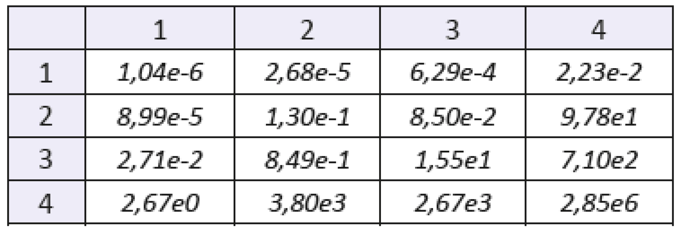
Table 2. The mixed statistical moments with f(x,y) of order 2. Sample: gelatine. The number of the row denotes order of coordinate “x”, the number of the column denotes order of coordinate “y”. 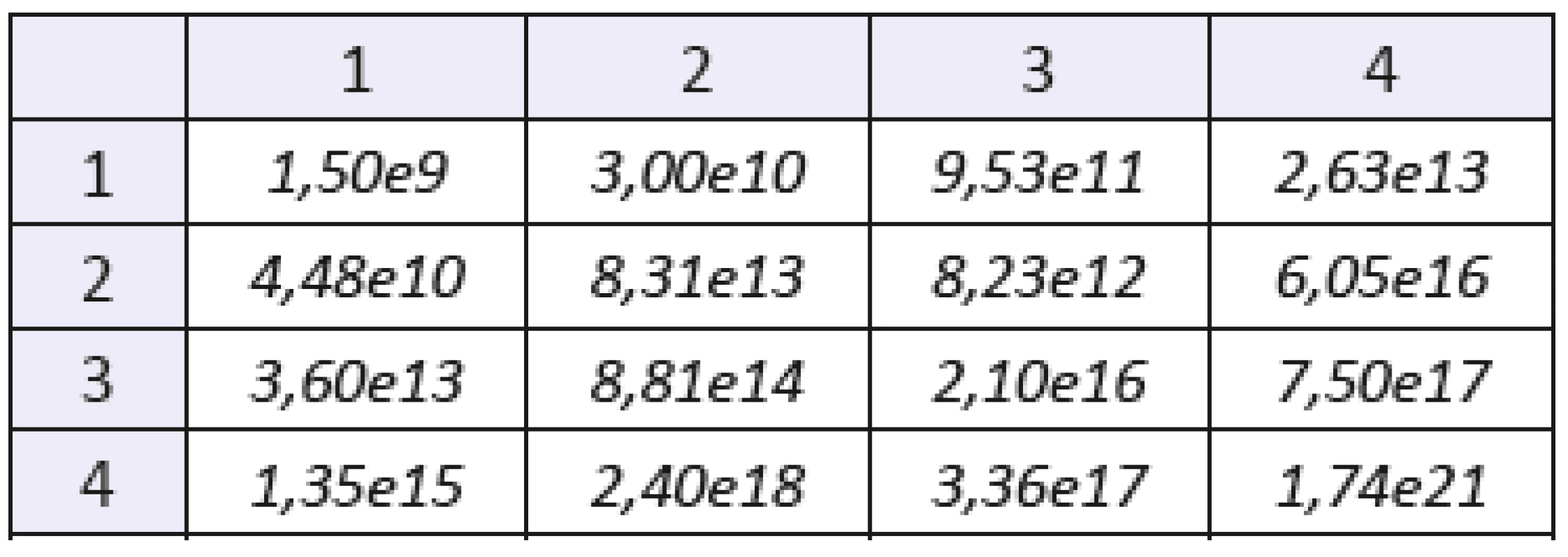
Table 3. The mixed statistical moments with f(x,y) of order 1. Sample: gelatine with lesser concentration of blood. The number of the row denotes order of coordinate “x”, the number of the column denotes order of coordinate “y”. 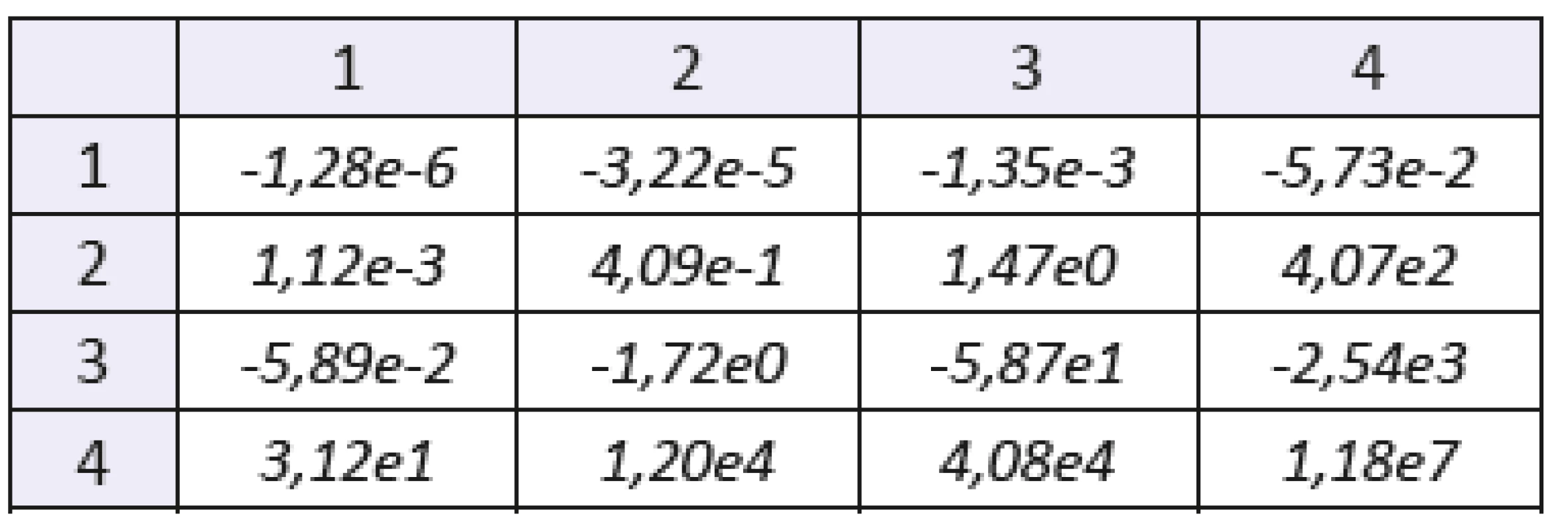
Table 4. The mixed statistical moments with f(x,y) of order 2. Sample: gelatine with with lesser concentration of blood. The number of the row denotes order of coordinate “x”, the number of the column denotes order of coordinate “y”. 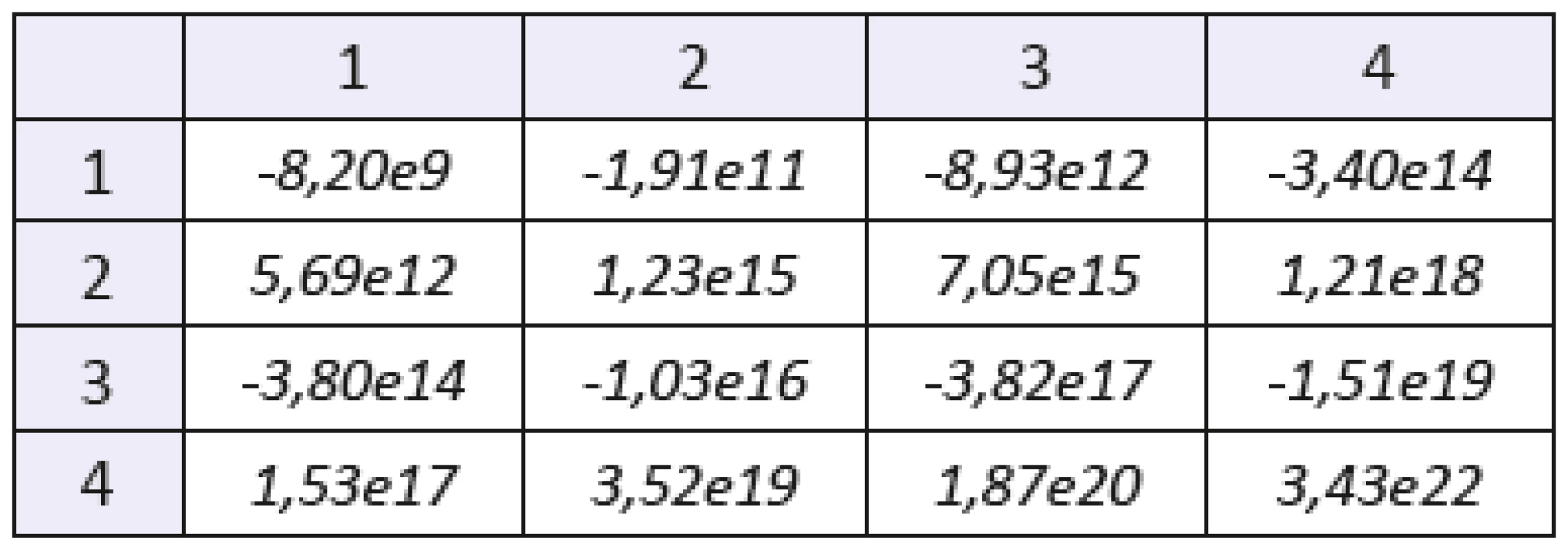
Table 5. The mixed statistical moments with f(x,y) of order 1. Sample: gelatine with higher concentration of blood. The number of the row denotes order of coordinate “x”, the number of the column denotes order of coordinate “y”. 
Table 6. The mixed statistical moments with f(x,y) of order 2. Sample: gelatine with higher concentration of blood. The number of the row denotes order of coordinate “x”, the number of the column denotes order of coordinate “y”. 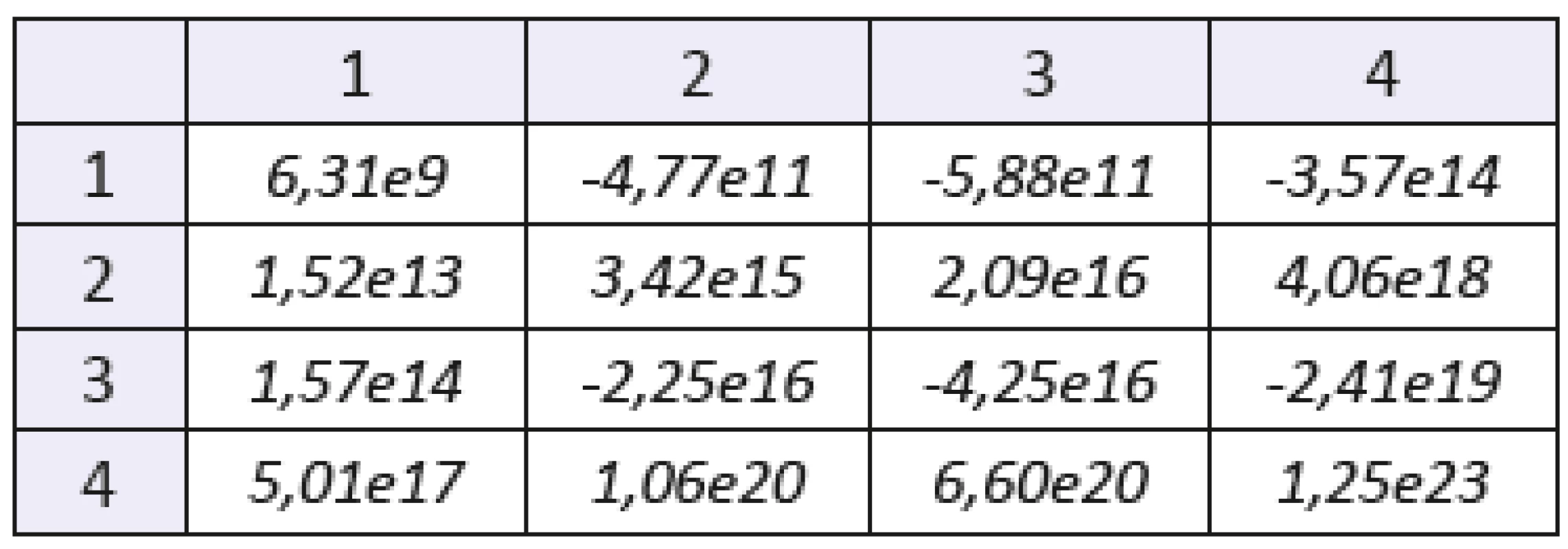
Table 7. The coefficient of variation of mixed statistical moments with f(x,y) of order 1. The number of the row denotes order of coordinate “x”, the number of the column denotes order of coordinate “y”. 
Table 8. The coefficient of variation of mixed statistical moments with f(x,y) of order 2. The number of the row denotes order of coordinate “x”, the number of the column denotes order of coordinate “y”. 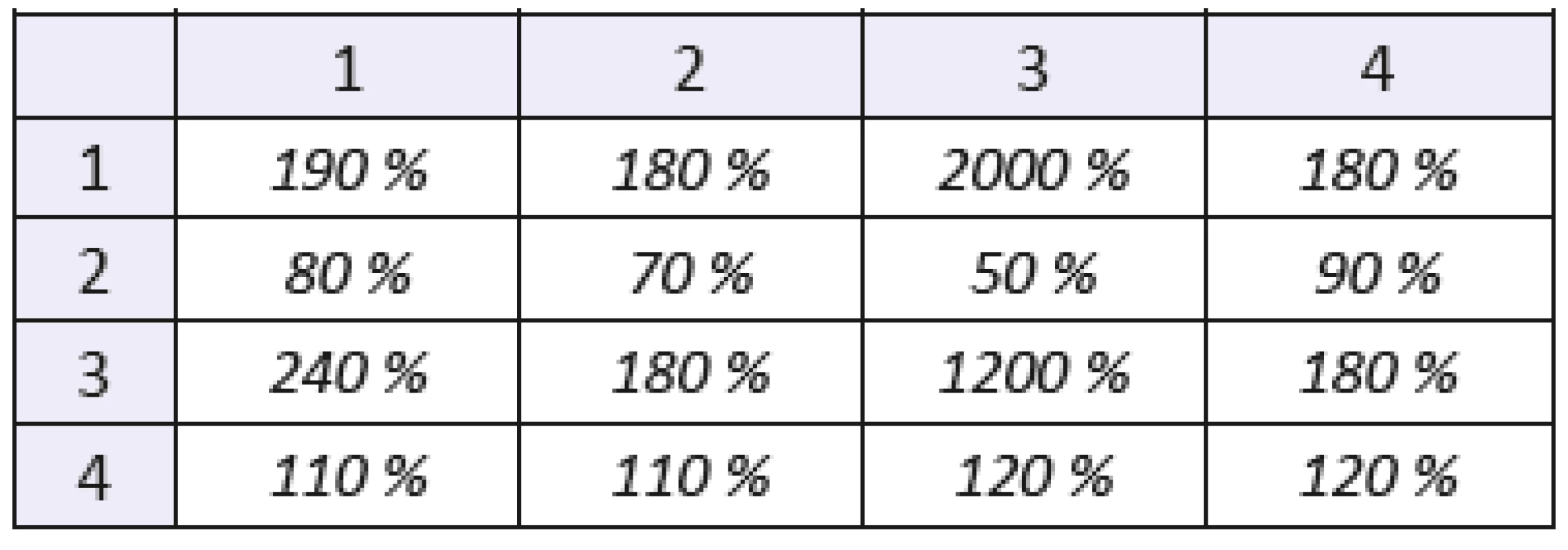
Conclusion
We have found that statistical moments of texture are capable of the use in texture analysis of medical ultrasound images due their high variation. Although we have analyzed only three samples, the range of values exceeds in some cases. Unfortunately, it is likely that statistical moments of texture and texture features derived from statistical moments will depend strongly and sensitively on factors such as a gain, a quality of probe, a processing of radiofrequency signals, and an image preprocessing. Some of those factors can be fixed and thus can be corrected whilest some other are something like “dwarfs inside a black‑box” of each ultrasound device and thus there are inaccessible for common users. Question about reproducibility of moment-based texture features of ultrasound images is challenge for further research.
In other hand, the simplicity of moment-based texture features may be useful in tasks about image segmentation in cases of adaptive segmentation which should be independent on a device and a setting of device especially in real‑time tasks.
In addition, we have found that mixed moments with symmetrically changed axes are usually different. This may be written mathematically:
From equation 8 may be derived family of texture measures which describe anisotropy of texture. These measures may be useful in some cases, but there is a broad family of rotation invariant texture features which are based on different principles. [10] Question about measurement of texture anisotropy in medical ultrasound remain for further research.
MUDr. Jaromír Šrámek
Department of Biophysics
Faculty of Medicine
Masaryk University in Brno
Kamenice 126/3, CZ-625 00 Brno-Bohunice
E-mail: formol@med.muni.cz
Phone: +420 728 151 326
Sources
[1] Azhari, H. Basics of ultrasound for engineers. John Wiley & Sons – IEEE Press, 2010 1st ed.
[2] Raeth, U., Schlaps, D., Limberg, B., et al. Diagnostic accuracy of computerized B-scan texture analysis and conventional ultrasonography in diffuse parenchymal and malignant liver disease. Journal of Clinical Ultrasound, 1985, vol. 13, p. 87-99
[3] Castellano, G., Bonilha, L., Li, L.M., Cendes, F. Texture analysis of medical images. Clinical Radiology, 2004, vol. 59, p.1061-1069.
[4] Gonzaes, R.C., Woods, R.E. Digital image processing. 3rd ed Pearson Pretice Hall 2008.
[5] Velho, L., Frery, A.C., Gomes, J. Image processing for computer graphics and vision. 2nd ed., Springer 2008.
[6] Shalizi, C. Continuity of stochastic processes. Url: http://www.stat.cmu.edu/~cshalizi/754/notes/lecture-07.pdf
[7] Dupač, V., Hušková,. M. Probability and mathematical statistics. Karolinum 2005 [in czech].
[8] Erol, B., Kara, T., Gürses, C. et al Gray scale histogram analysis of solid breast lesions with ultrasonography: can lesion echogenicity ratio be used to differentiate the malignancy? Clinical Imaging 2013 [8 July, in press].
[9] Sarti, A., Corsi, C., Mazzini, E., and Lamberti, C. Maximum likelihood segmentation of ultrasound images with Rayleigh distribution. IEEE Transations on Ultrasonics Ferroelectrics and Frequency Control, 2005, vol. 52, no. 6, p. 947-960.
[10] Manthalkar, R., Biswas, P.K., Chatterji B.N. Rotation invariant texture classification using even symmetric Gabor filters. Pattern Recognition Letters, 2003, vol. 24, p. 2061-2068.
Labels
Biomedicine
Article was published inThe Clinician and Technology Journal

2013 Issue 2-
All articles in this issue
- WEARABLE ARTIFICIAL KIDNEY – EVOLUTION OF ITS CONCEPTS AND CURRENT STATE-OF-THE-ART
- On mixed statistical moments of texture in ultrasound B-mode images
- Artefakty spôsobené pacientom pri zobrazovaní magnetickou rezonanciou
- Indikace k operační léčbě popálenin při využití metody laserdoppler imaging
- Aj všeobecní lekári si budú môcť aktualizovať profesné kompetencie pomocou medicínskych simulátorov (výhody a úskalia)
- Hodnocení revaskularizace dolních končetin pomocí termografických měření a metodika
- The Clinician and Technology Journal
- Journal archive
- Current issue
- Online only
- About the journal
Most read in this issue- Artefakty spôsobené pacientom pri zobrazovaní magnetickou rezonanciou
- Hodnocení revaskularizace dolních končetin pomocí termografických měření a metodika
- Indikace k operační léčbě popálenin při využití metody laserdoppler imaging
- WEARABLE ARTIFICIAL KIDNEY – EVOLUTION OF ITS CONCEPTS AND CURRENT STATE-OF-THE-ART
Login#ADS_BOTTOM_SCRIPTS#Forgotten passwordEnter the email address that you registered with. We will send you instructions on how to set a new password.
- Career


